|
E x a m p l e s
|
|
I assume here that you have advanced in your GEOP 205 to where you are familiar with some of the basic solutions of LIP (Linear Inverse Problem). In this page I present some simple but important examples of LIP that illustrate some of the important features of the different inverse problems encountered in geophysical interpretations work.
1. The Dampened Least Squares Problem:
The objective of this example is to illustrate the computational mechanics of this important type pf solution to the inverse problem. Recall that the damped least squares solution is derived under a combination of criteria:
(1) Minimum prediction error
E(m) = (G m - dobs)T (G m - dobs)
(2) Minimum solution length:
L(m) = mTm
The objective function to minimize, therefore is:
q(m) = E(m) + m L(m)
Which yields the solution:
mest = [GTG + m I]-1 GT dobs
We generate a set of synthetic data from a quadratic model: y = a + b x + c x2 .
Here is the MATLAB® script to do so:
|
mtrue = [10.0 3.5 -2.89] |
|
% True Model Parameters |
|
x = [-3:.1:3]'; |
|
% Note the sampling rate dx = 0.1; |
|
d = p(1) + p(2)*x + p(3)*x.^2; |
|
% Generate error-free synthetic data d |
|
er = randn(size(d)); |
|
% Generate Gaussian random error |
|
er = (er - mean(er))/std(er) |
|
% Standardize error to white noise with mean = 0 and var =1 |
|
dobs = d + er; |
|
% Form observation data vector with errors. |
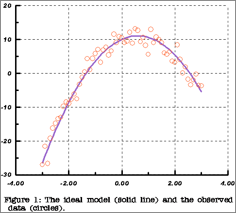
Figure (1) to the right shows our model together with the noisy observations. Our objective is to attempt to recover estimates of the model parameters m = [10, 3.6, -2.89] from the noisy observational data dobs .
Here is how we may form the design matrix G:
G = [X.^0 X X.^2];
The first 4-rows of G:
1.00 -3.00 9.00
1.00 -2.90 8.41
1.00 -2.80 7.84
1.00 -2.70 7.29
We want to solve the problem for several values of the dampening parameter m and save the results of each solution for examination and comparison. We do so via a for-loop as follows:
for k = 0: 0.1: 1;
n = 10*k+1;
H= (G' * G + k * I)
D = G' * do;
M(:,n) = H\D;
end;
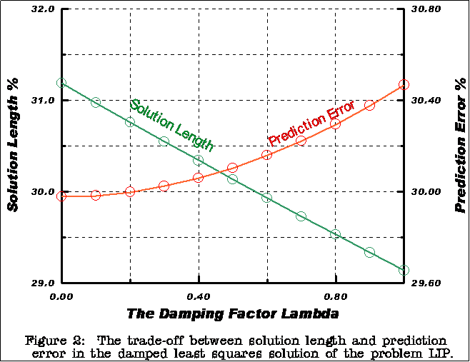
The results are shown in Figure (2), which illustrates the trade-off between minimum prediction error E and minimum length solution L as the damping factor m increase towards unity.
![]()
2. Delay Time in Seismic Refraction Surveys
![]()
The concept of delay time is important in the interpretation of refraction seismic data, especially in the Hagedoorn plus—minus method of interpretation. In this method, it is assumed that the layers present are homogenous, that there is a large velocity contrast between the layers, and that the angle of dip of the refractor is less than 10o. The method uses intercept times and delay times in the calculation of the depth to a refractor below any geophone location. Referring to Figure (1), the delay time (Dt) is the difference in time between:
the time taken for a ray to travel along a critically refracted path from the source via the sub-surface media and back to the surface (TABCD along the path ABCD);
the time taken for a ray to travel the equivalent distance of the source-geophone offset (x) along the refractor surface (i.e. TPQ along the projection PQ of the refracted ray path onto the refractor surface).
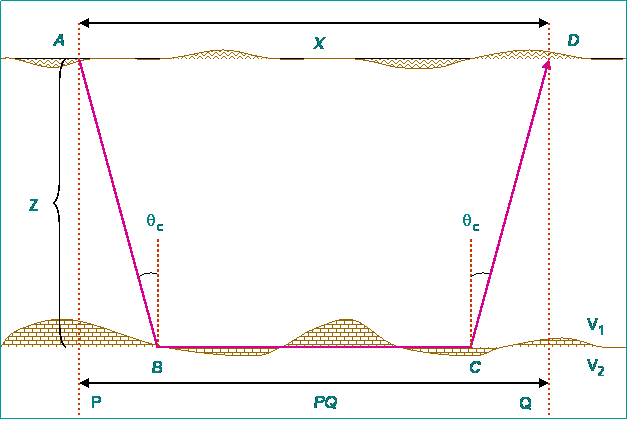
The total delay time Dt is effectively the sum of the ‘shot-point delay time’ (Dts) and the ‘geophone delay time Dtg. In cases where the assumptions on which the method is based are realistic (especially the refractor dip is not too large), it is sufficiently accurate to consider the distance PQ to be approximately the same as the source-geophone offset X. The mathematical equations relating the various delay times and velocities are then as follows:
The total delay time is:
Dt = TABCD - TPQ
TABCD = (AB + BD)/V1 + (BC)/V2 and TPQ = PQ/V2
Thus
Dt = (AB +CD)/V1 - (PB + CQ)/V2 = (AB/V1 - PB/V2) + (CD/V1 - CQ/V2)
= Dts + Dtg ~= TABCD - x/V2
Or, setting TABCD = t
t = x/V2 + Dts + Dtg
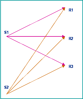 Consider now the refraction delay time experiment shown in the figure
to the right, where two shots are received at three stations each. Assuming a two-layer
Earth model with velocities V1 > V2 for the top and bottom layers respectively,
then the travel-time between shot (i) and receiver (j) is:
tij = s2 x + εi + δj
Where S2 is the slowness of the refractor (= 1/V2) and are the delay times associated with the shot points and receivers respectively. The matrix formulation of this problem is of the form:
d = G m

Note the special structure of the G-matrix of this problem. Many of its elements are zero and ones. This is called a sparce matrix and is of special importance in geophysical computations.
![]()
3. Travel Time Seismic Tomography
![]()
Tomography is the process of obtaining a 2 and 3D images of a slice through the
interior of a 3-dimensional object by passing rays of some sort through the
object and observing how the rays are affected (attenuated or delayed in time)
by passage through the material.
There are applications of tomographic imaging in many different fields. In medicine, methods include X-ray tomography, ultrasonic tomography, magnetic resonance imaging, and positron emission tomography (PET). In the earth sciences, tomography is widely used In seismic and EM imaging. In cross-well seismic tomography, for instance, acoustic waves are generated within one well, and received by sensors in a second well. In cross well radar tomography, ground penetrating radar waves (at frequencies of hundreds of MHZ) are used. In seismic tomography of the deep earth, seismic waves from naturally occurring earth quakes are sensed at stations on the surface of the earth. Tomography techniques are also used in the analysis of controlled source seismic data generated by reflection of seismic waves from geological structures.
Tomography depends on the assumption that energy from the transmitter follows ray paths through the 3-dimensional body to receivers. Under this assumption we can evaluate path integrals along ray paths to determine travel times and attenuations. Of course, computing the travel time or attenuation from the known physical parameters of the 3-dimensional problem is a forward problem. What we want is to determine the physical parameters which result in the observed travel times or attenuations.
In the simplest case, ray paths follow straight lines with essentially no refraction (bending rays) or diffraction (scattering from small features). The problem becomes nonlinear and much more difficult as we consider refraction effects which result in curved ray paths, and especially when we consider diffraction effects. The straight ray tomography problem, however, can be formulated as a linear inverse problem that can be addressed using the techniques that we introduce in GEOP 205.
|
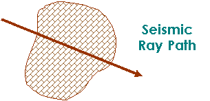
In this example, we consider the simple straight-ray travel time tomography problem and formulate it as a linear inverse problem. A seismic ray passes through a 3-D object as shown in the figure to the right. The travel time through the object is given by the line integral:
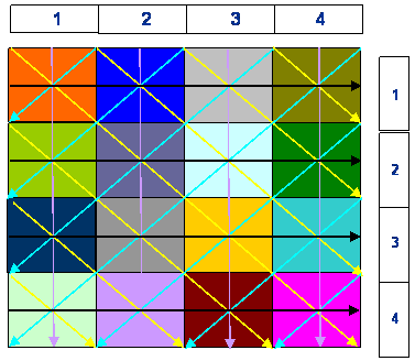
where S(x) is the seismic slowness (1/velocity) of the object. In practice, we evaluate the line integral numerically by discretizing the object into blocks of dimension Δl, and assume that S(x) is constant in each block as is shown in figure for 9 blocks. This allows us to write the travel time approximation: |
 |
|
 |

which leads to a set of linear equations of the form G m = d.
Now consider a simple tomographic experiment in which we discretize the object into a 4 x 4 blocks. If we use 4 E-W and 4 N-S rays, we get a rough image of the target; more details may be obtained if additional diagonal scans are performed. Here is how the equations for the first row and first column scans look like:
t1 = ( s11 + s12 + S13 + S14 ) Δl
t5 = ( s11 + s21 + S31 + S41 ) Δl
For the diagonal scans, the equations are not as easy to code; and things get even messier when considering radial scans. Here is the equation for the main diagonal scan:
t11 = ( s41 + s23 + s32 + S41 ) Δl
I am sure that with this equation and the figure above, you can write down the equations for all diagonal scans of the image.
Now that we know the basics of tomography, let us setup a simple tomography problem and try to work out its solution. The objective of this exercise is to illustrate again that important Geophysical Inverse Problems are not easily solvable. They have innate characteristics of being under-determined, ill-posed and unstable. Hence, they require special algorithms to handle them properly.
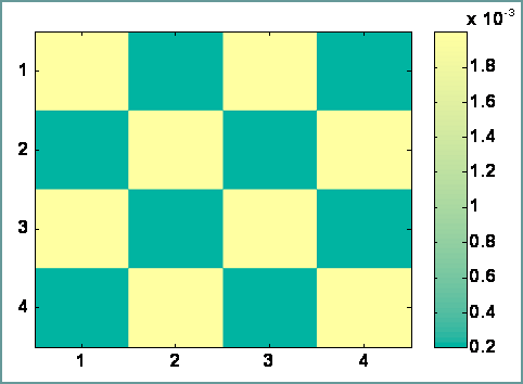 We
select for our problem the target image of the checkerboard shown in the figure
to the right. This is the matrix of slow nesses of the various blocks that
make up the object. We have intentionally selected a situation of high velocity
contrast (~ 100 m/sec) between adjacent blocks just to make the problem somewhat
simpler to solve.
Here are the steps to follow to generate synthetic data and set up the problem:
Construct the design matrix G;
Using a set of 16 velocity values, convert to slowness st (call this the true slowness vector);
Compute synthetic arrival-times data dt (true data) from: dt = G st
Here is how your [22 x 16] G-matrix should look like assuming you have followed the scan sequence:
Row => Column => NE-SW => NW-SE. This sequence determines the arrangements of your equations and consequently the structure of the G-matrix.
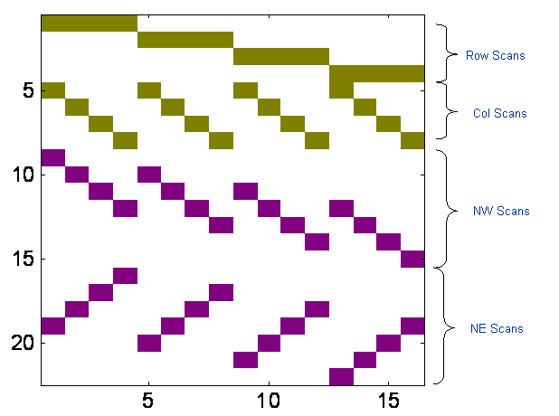
Colored matrix elements (pixels) contain values of 1 or √(2); all others (white background) contain zeros. This indeed is a special type of matrix that we may expect to give us some problems when attempting to invert it. How would we know the quality of G-1 ? Find the condition number, or rank or the SVD of G. The appropriate MATLAB commands return:
cond(G) = 9.7892e+015 rank(G) = 15 .. .. ooops! i.e. rank deficient (= singular).
Let us look at the SVD of G; the command [U S V] = svd(G) returns:
diag(S) = [...., 244.95, 244.95, 218.84, 200.00, 200.00, 200.00, 141.42, 141.42, 116.33, 000.00 ]
So, the 16th singular value is ZERO. This says that we can not
expected to recover the image from direct inversion or simple Least Square
solution. We have to try other techniques that will allow inversion to proceed
without destabilizing the computation to a disastrous end! There several such
techniques developed specially for tomographic imaging of which are the so
called ART, KAC and SIRT methods. These inversion strategies were developed
specially for seismic tomography and subsurface imaging. In the figure below are
the solutions obtained by direct (un-regularized) and by Damped Least
Squares. You can see for yourself what works best!
|
|
| Comparison of simple Least Squares and Damped Least Squares solutions to the checkerboard tomography problem |
If you find this problem interesting and/or challenging, here is a collection of MATLAB functions TOMO that will generate the G-matrix for the 4 x 4 image and the horizontal, vertical and diagonal scans. It also includes solver functions of all the three methods mentioned above (ART, KAC and SIRT) and an additional method (not discussed here) called TOTAL Least Squares. Experiment with them under different conditions of random errors, scan sequence, etc.
Have FUN
![]()