|
Basic Concepts and Definitions
|
|
What is Inverse Problem?
In General: Roughly speaking, Inverse Problems could be described as problems where the answer is known, but not the question; or where the results, or consequences are known, but not the causes.
For example, if 3 streams join to form a river, and we know that 3 factories are putting known amounts of pollutant into the streams, then we can calculate the resultant pollutant in the river. This would be the forward, or classical problem. But a more likely problem is that we only know the pollutant in the river, and we have to establish which factory is putting what into which stream. This is the inverse problem.
As another, simpler example, If you know the specific heat capacity of a liquid, you can calculate, for instance, how long it will take to boil a given quantity of the liquid. Now suppose you know how long the liquid takes to boil, can you tell what liquid it is?
You can see the problem has become more complex, especially if more than one liquid share the same specific heat capacity. This is probably the reason why you don't come across inverse problems in traditional education. This is not a drawback of education as such, it is just that these problems are not easily 'packaged' into a set of question and answer problem.
In Geophysics: More formally, however, we say that Geophysical Inverse Problem is the problem of making inferences about physical parameters of Earth systems from observational data. To accomplish this task, we rely heavily on an organized family of mathematical techniques and philosophies that makeup the body of Inverse Theory.
Since nearly all data are subject to some uncertainty, these inferences are usually statistical. Further, since one can only record finitely many (noisy) data and since geophysical systems are usually modeled by continuum equations of physics, no geophysical inverse problem is really uniquely solvable: if there is a single model that fits the data there will be an infinity of them.
An Elementary Geophysical Inverse Problem
![]()
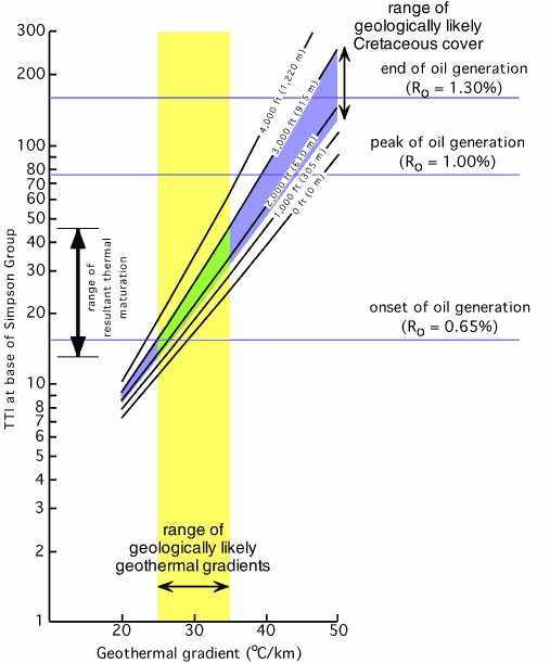
 Thermal regimes and regional fluid flows are critical factors in the formation
and maturation of petroleum, gas and coal deposits.
The figure to the right is a sketch of the petroleum window limited by the
geothermal gradients appropriate for the formation and accumulation of oil
deposits in a given area.
Suppose you are assigned the task of determining the geothermal gradient in Alghawar oil field from one of its deep wells. Here is how you probably may proceed:
Get your gear (thermal probe and depth measuring device) and head to the target well;
Make measurements of of the temperature T (oC) in the borehole at regular intervals of depth, say Dz = 100 meters;
Get back to the office and begin the chore of numerical computation;
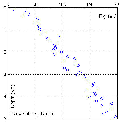
The starting point is to plot the temperature measurements (OBSERVATIONS or DATA) vs depth which may look as is shown in Figure 2. Clearly the relation between depth and temperature is a linear one, so that you may choose a straight line as the system model. That is to say the physics of the problem at hand is such that:
T = a + b z; MODEL. .. .. .. .. Eq(1)
In ordinary situations, we know the numerical values of [a, b], and by inserting a set of depth (z) values we compute the corresponding
temperatures (T) at each depth; thus we go from right to left of the model equation.
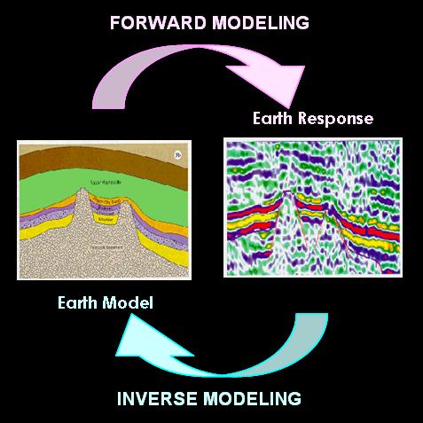
This is the FORWARD PROBLEM or
FORWARD MODELING. T-values computed in this
manner are calle d PREDICTED data or model
RESPONSE.
The situation at hand, however, is quite different. We have already spent time in the field to measure temperatures T at predetermined set of z-values. We seek now to find the numerical estimates of [a, b], the MODEL PARAMETERS that will best-fit the observational data. This is the essence of the inverse problem. We want to proceed from right to left in the model (see Figure 3 below). This brings us to the next task in our computational agenda.
Formulation of the Inverse Problem
![]()
|
In the table to the left, we show the first 10 measurements of the temperatures that were made from the well at Algawar. By selecting Eq.(1) as our model, we are implicitly asserting that there is a set of model parameters [a, b] such that for every depth value listed in the Table, they yield the corresponding temperature measurement observed in the field. Hence, we may write the following set of equations: T(i) = a + b z(i), for i = 1, 2, 3, .. .. .. , N If we place all the T-values (our observed data) in a column vector, d = [T1, T2, T3, .., .., .., TN]T; and place the model parameters in another column vector, |
z (km) |
T oC |
|
0 |
20.6744 |
m = [a, b]T; (the superscript T stands for matrix transpose)
then we may write the set of equations in matrix form as:

where,

or,
d = G m
This is the inverse problem that we need to solve to complete
our GTG project for the Oil Company. Note that in the equation above both the
data (d) and the model
parameters (m) are in separate
vectors of their own. This is the main feature of the so-called Explicit Linear Inverse Problem (LIP). Other types of inverse problems are:
Implicit linear problem of the form:
d = g(m)
Non-linear problem of the form:
F(d, m)=0
In geophysics we deal mainly with the explicit linear problem; if our actual problem is not of this form, we resort to some methods to reduce to LIP by linearization.
There are many different points of view regarding what constitute a "solution" to an inverse problem. If one merely wants to know the numerical values of the model parameters, then the problem becomes one of estimation. Very infrequently, however, is it possible to solve an inverse problem in such a way as to obtain this kind of exact information.
Instead, we are often forced to make compromises between what information we desire to get from a solution and the kind of information that in fact is contained in the data. These compromises lead to other kinds of "answers" that are less direct than parameters estimates. Indeed a major part of the practice of inverse theory is to identify what features of a solution are most valuable and then make the compromises that help emphasize these features. we devote a considerable part of this course to this aspect of Inverse Problem.
Some Application Areas of Inverse
Theory
![]()
Data fitting;
Image enhancement;
Digital filter design;
Deconvolution of seismograms;
Determination of earth structure;
Modeling and estimation in mineral prospecting;
Determination of earthquake location;
Modeling of lithosphere’s response to loading or strain rate variations in sedimentary basins;
Well (pump) test analysis in hydrogeology;
Factor analysis in geology;
Geochronological determinations using geomagnetic reversals data;
Satellite navigation;
Optimal control of engineering systems;
Seismic and Medical tomography;
Decision making;
Operational research in management and mineral economics.
Geophysical Processes
and Systems
![]()
Seismic or electromagnetic wave propagation through the earth and current or fluids flow in porous rocks are examples of Geophysical Processes. The Earth may be described in terms of its physical property distributions which define various physical systems that may be investigated by observing say, wave propagation in the subsurface. Examples of Geophysical Systems include:
Density distribution within the Earth.
Velocity distribution within the Earth.
Temperature distribution within the Earth.
Resistivity distribution within the Earth.
Distribution of radioactive materials within the Earth.
Magnetic susceptibility variations within the Earth.
Useful Links
![]()
These are some of the richest sites I know of that
are dedicated to various aspects of geophysical inverse problem. The site at UBC has several highly rated online tutorials on different inverse problems of
geophysical exploration. AT SEP you will find several excellent
FREE eBooks on
various topics of geophysical imaging and seismic modeling and inversion.
|
|
||
|
|
||
|
|
||
|
|
||
|
|
||
|
|
||
|
|
||
|
|
||
|
|
||
|
|
![]()