Let us look at some light brain teasers of inversion.

Teaser 1:

A zoo-keeper, when asked how many birds and animals were in his care, replied, "I have one hundred heads and three hundred feet." How many of each did he indeed have in his care?

As a good students of algebra,  you take out your pen and calculate:

a = Animals               b = Birds

a + b = 100 ,              for the heads

4 a + 2 b = 300,         for the feet

Which yields:             a = 50    and    b = 50.

Simple . . . . you say, two equations are sufficient to determine two unknowns. . . ..  Sometimes may be, but not always!

Suppose now that the  zoo contained only animals, say  lions (L) and tigers (T), and the keeper again reported 100 heads and 300 feet,

L + T = 100                           

4 L + 4 T = 300, or L + T = 75

These two equations are clearly contradictory. The keeper is misinforming us!

If on the other hand the keeper reported 100 heads and 400 feet, then with L lions and T tigers the equations would be:

L + T = 100

4 L + 4 T = 400

 These equations are now redundant and, hence, do not provide enough information to separate the values of L ant T.

Teaser 2:   

Consider the following problem of simultaneous equations:

x + y = 2

2 x + 2.000001 y = 4.000001

The solution simply is:        x = 1.0    and    y = 1.0

Now let us ignore the small fraction on the RHS, so that the equations are written as:

x + y = 2

2 x + 2.000001 y = 4.0

The answer becomes:    x = 2    and     y = 0;      Quite different!

If on the other hand we ignore the small fraction on the LHS so that:

x + y = 2

2 x + 2 y = 4.000001,

then any attempt to solve the problem will lead to an absurdity: 0 = 0.000001!

Finally, if we ignore the fraction on both sides so that:

x + y = 2

2 x + 2 y = 4,

then the two equations are redundant and do not provide sufficient information to solve the problem.

It is a common belief that "computers do not make mistakes".  Well this is only a misconception. In fact computers make silly (and some times serious) mistakes. Therefore, we must learn how and when they make such mistakes so that we may properly evaluate the quality of our computational results.  

Examine the MATLAB function below.

Now, if we add the fraction 0.0001 to itself 10000-times we should expect the result to be 1.0, no more no less.  Let us find out if computers understands that much simple arithmetic:

y=roundoff(0.0001,10000)

y = 9.999999999999062e-001 

 Close but not exactly! The percent error is:

pe = 100 x (1.0 - y)/1.0 = 9.381384558083453e-012

We may evaluate the significance of this seemingly small error in two ways:

1. We compare it with the machine zero, which is different from true zero (0). It is called the machine EPSILON. In MATLAB command window, enter the command eps to get:

2.220446049250313e-016.

This number is  recognized by your computer as its zero. That is for any real number x :

   x + eps = x.

Comparing the percent error with the machine epsilon we get:

pe/eps = 4.225000000000397e+004
 That is the error is 4-orders of magnitude greater than the machine epsilon, considerable to be sure.

2. To further appreciate the seriousness of the error, let us use y above in the further computations:

A = 1.0;         C = 5.0E+16;        D = (A - y)*C.

Ideally D = 0. The actual result, however, is far from that. It is:

D = 4.690692279041286e+003

Not only did the small error propagate in subsequent computations, but it has also been greatly magnified. The relative error in D is infinite!

Let a be an approximation to an exact quantity x, then:

        The absolute Residual is:    |x - a|

        The absolute relative Error: |(x - a) / x|

Insight into the nature of relative errors may be gained by examining the following table for the possible approximations a to x = 3.526437:

Examination of the relative error in the table above suggests the following rule of thumb:

If the relative error in the approximation a is of order 10^-n , then a and x agree to about the n^th significant figure, and conversely.

Analysis of round-off errors is made possible from knowledge of their bounds in Floating Number Systems (FNS) employed in most computers. If we think of computer representation of exact quantities x via FNS as a mapping (function) FL(x) = a, where, a = FNS representation of x, then for a n-digit precision computation we may write:

Clearly addition introduces the largest error compared to other operations.

Example 1:   

Find the smallest root of the quadratic equation:

 x² -  6.433 X + 0.009474 = 0

 For a = 1.0, b = -6.433, and c = 0.009474, we apply the well-known expression:

x = {-b ± SQRT (b² - 4ac)} / 2a

x₁ = {6.433 - SQRT [(6.433)² - 4(0.009474)]} / 2

The answer to 5-figure accuracy is:     x₁ = 1.4731 x 10^-3.

However, assuming a 4-digit precision computer, the computation may proceed as follows:

Z is the FNS approximation to x₁. Thus, the computed result fails to agree with the true value in the second significant figure. The relative error is -0.0183.

Example 2:   

Solve the following simultaneous equations:

 3.0  X + 4.127 Y = 1.541

1.0  X + 1.374 Y = 5.147

 The answer to 6-figure accuracy is:

X = 13.6658        Y =  - 6.2000.

Using our 4-digit precision computer, the computation may proceed as follows:

y =[ 5.147 - (15.41/3) ] / [1.374 - (4.127/3)]

Despite their similarities, computations in the two examples above fail for quite different reasons. In the first example, failure is mainly due to the use of the familiar expression of quadratic equations roots which leads to cancellation of significant figures. A more accurate result may have been obtained using the alternate expression:

x₁ = 2.0 (0.009474)/{6.433 + √[(6.433)2 - 4 (0.009474)]},  which yields X₁ = 1.473, a perfectly satisfactory answer.

The problem of the second example, on the other hand, can not be solved accurately in 4-digit FNS no matter how we rearrange the computations. In fact a slight perturbation by rounding of the Y-coefficient in the first equation renders the problem inconsistent and unsolvable!

In short, the difference between the two examples is that the first illustrates a bad way (Algorithm) of solving a reasonable problem, whereas the second presents a poorly posed (ill-posed or ill-conditioned) problem.

Loosely speaking a problem is said to be ill-posed if the solution is sensitive to errors in the data such that small changes in the data can cause arbitrarily large changes in the results.   Such problems arise in a wide variety of important applications, including remote sensing, medical imaging,  environmental modeling and most notoriously integral equations of the first kind which are the commonest  in applied geophysics. ill-posed problems require special solution methods, the most widely used of which is regularization.

An effective tool for the numerical analysis of ill-posed problems is the so-called SVD (Singular Value Decomposition) which we will discuss in the next section, but first here is a formal definition of ill-posedness or ill-conditioning.

Definition:

Let X* be an approximation of X, and y = F(X), for some function F;  if F(x) is significantly different from F(X*), then the problem is said to be Ill-Conditioned.

We begin by recalling some basic concepts from Linear Algebra.

Vector Norms

First let us understand the concept of vector norm which plays a central role in Inversion Theory. You must be familiar with the idea of vector length. Given a 3-D vector V, its length or magnitude |V| is computed as:   |V| = √(v_x² + v_y² + v_z² ).

Now what is the length (norm) of an n-dimensional vector? Here is the most general definition of the  norm of an n-vector - called the L_p - norm:

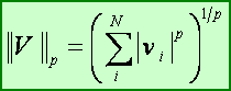
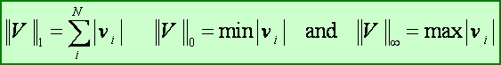
The familiar vector norm corresponds to p = 2, and is called the L₂ - norm. Two other important norms are: L₁ , L₀  and the L_∞ norms and are respectively defined by:

Eigenvalues and Eigenvectors

Another important concept relevant to inverse problems is that of eigenvalues and eigenvectors (eigen = German meaning proper). Usually when a matrix G operates on a vector x it changes its direction and magnitude. But there is a special class of vectors, eigenvectors, such that the action of G is merely to scale them leaving their directions unchanged. Mathematically this fact is expressed as:

for some constant l. The eigenvectors x (possibly several) of the matrix G and their corresponding eigenvalues l (possibly several and distinct) are usually found by solving the set of homogenous equations: (G - lI) = 0, which, for non-trivial solution requires that: |G - lI| = 0. Now we are ready to introduce the following important result from Linear Algebra:

Singular Value Decomposition of a General Matrix

During the past two decades much interest has been given to the application of Singular Value Decomposition to a wide range of geophysical inverse problems from parameters estimation to modeling and digital signal processing. SVD provides a powerful tool for analyses and solution of rank deficient and ill-conditioned inverse problems.

Let us see how SVD works starting with a simple even-determined (N x N) problem:

This is the forward problem which we may think of as a mapping from model-space m to data-space d.  It is safe to say that there is some orthogonal matrix V (to be found) that maps the model (m) and data (d) vectors into new model and data vectors M and D respectively such that:

Substituting back into equation (1) we get:

The matrix V always exists and is an [N x N] matrix whose columns are the normalized eigenvectors of G. Moreover, S = [V^T G V] is an [N x N] diagonal matrix whose main diagonal elements are the eigenvalues of G. In terms of S and V, the solution of the inverse problem is given by:

or in expanded form:

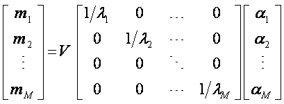
or more explicitly:

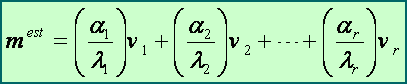
where    a = V^T d^obs  . Thus, from an examination of the eigenvalues of G, one can tell at a glance whether a reliable estimate can be obtained from d^obs and G!

The solution vector m^est  is seen to be a weighted sum of the parameter eigenvectors v_i with weights a_i / l_i. In particular, if a_i/l_i is small, then the term (a_i/l_i)v_i  has relatively little influence on the solution m^est . More important, however, is when any l_i is very small; in this case a_i/l_i will tend to be very large, so that any errors in the data will be amplified and propagated to the solution via the terms a_i , thus rendering the entire computation unstable and the solution meaningless!          

Following is the main theorem of Linear Algebra  that generalizes the SVD tool:

Some important properties of SVD include:

1. The rank r of G is the number of the non-zero singular values. A rank-deficient [N x M] matrix G is a singular matrix and is such that:     Rank(G) < min(N, M).

2. The condition number of G is the ratio of its largest to smallest non-zero [i.e. > EPS] singular values:

 Cond(G) = l₁ / l_N  ≥ 1.0

Thus, the larger the condition number of a matrix, the more near-singular  or ill-conditioned it is.

Example:   

Let us revisit our second brain-teaser and examine its SVD structure to pinpoint where the problem lies.

We resort to SVD analysis to answer important questions about the inverse problem such as:

In matrix form, the problem is stated as follows:

d = G m

where:

Remember that the Least Squares solution to this problem is simply:     m^est = [1.0,  1.0].

In MATLAB^® command window, enter the command:    [U S V]=svd(G), and examine S:

Note how small the second singular value is compared to the first. Suppose that the second datum is perturbed by an errors:  e= 0.000001(or 1.0 E-6), so that the new data vector is:   

The solution in this case is:     m^est  = [2.0,  0.0], which is useless!

What happened? How could such a small error in the data cause the inversion to fail?

Well, to begin with the error e, is small only in the eyes of the beholder but the computer. Compared to machine epsilon, the error is: e/eps ~= 0.450E+10. Moreover, this error is multiplied by the reciprocal of the second (and small) singular value l₂ of G to be propagated into the solution with magnification factor of ~ 3.16E+006. It is this magnifying power of small (near-zero) singular values that cause computational instabilities and lead to meaningless solution of inverse problems !

Now let us approach the problem from the Damped Least Squares point of view. As was discussed in class, the solution in this case is given by:

SVD analysis of this solution shows that the singular values of the inverse are terms of the form:

S(i, i) = (l_i + m). Thus, m stabilizes the computation even when the l_i's are very small or even zeros!

Use MATLAB to compute the Damped Least Squares solution from the perturbed d^obs =[2.0, 4.0], and for m = 0.0001.

You should get an answer of  m^est  = [ 0.99998960110816,  0.99998999910382], considerably more satisfying than the minimum prediction error solution.