Supply the arguments to the rkfixed command. The returned
values will be stored in a matrix we will call "s"
.
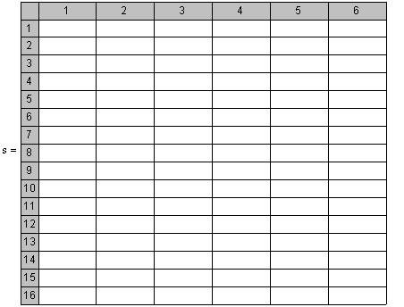
The matrix s will have 5 columns. Describe the content
of each column.
first column of matrix s =
2nd column of matrix s =
3rd column of matrix s =
4th column of matrix s =
5th column of matrix s =
Step 6: Display the matrix "s"
Part D
. (comparing the exact solution with the approximate
solution)
In this part of the project you will be asked to compare
the approximate solution returned by the rkfixed command
in part (C) of the project (column 2 of the matrix
appsol) with the exact solution obtained in part B
of the project.
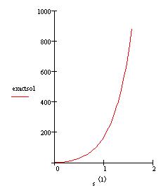
The exact solution of the IVP obtained in part B is
displayed for you below:
The rkfixed command has the form:
rkfixed = (ic, it, ft, Nsteps, D)
The five arguments of the command are:
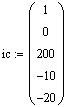
ic = a vector
containing the initial conditions
it = the first
value of the solution interval
ft = the last
value of the solution interval
Nsteps = number
of steps
D = the derivative
vector
Step 1: Define the vector with the initial values
Step 2: Define the initial and final point of the interval
Step 3: For the rkfixed we want the solution to be evaluated
at 51 points, so we use
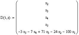
Use the substitution x1
= x, x2
= x', .... to transform the equation into a system
of first-order differential equations. Then
define the derivative vector used in the rkfixed command
Hint: If you do not know how to do it, see the file
040204ii-4.
mcd in the directory "I:\Common Files\software
literature\mathcad\040204ii-4.mcd)
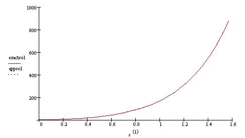
To get a visual comparison, fill-in the placeholders
"

" in the plot below with the appropriate names
to see the graph of the exact and the approximate solutions
Graph of the Exact solution
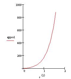
Graph of the Approximate solution
1. Compute the absolute value of the maximum error
between the approximate solution and the exact solution
2. Plot both the exact and the approximate solutions
on the same graph.
(Do not delete. This is used to reset the value of t)
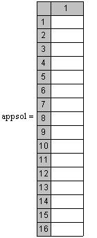
Name the approximate solution (column 2 of the matrix
s) appsol. That is, define column 2 of the matrix s
as "appsol"
Hint: Use the Vector and Matrix palette to extract a
matrix column
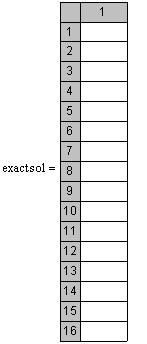
Evaluate the exact solution x(t) at the time steps returned
by the rkfixed command (the first column of the matrix
s) and define it as "exactsol".
Hint: You have to vectorize the evaluation. That is,

For comparison, the exact and approximate solutions
are displayed for you side by side below
Hint: If the matrices displayed below do not match,
it means that you did not do the right thing above.
Step 4: Write the general solution in terms of the constants
c1,.....,c5
The following symbolic computation will verify if your
answer above is correct. It will substitute your solution
into the differential equation and evaluates it symbolically.
If Mathcad returns a zero (after the arrow) then your
solution is correct. Otherwise, you have to reconsider
your solution.
Note: This area is locked so that you can not edit it.
Part B
. (finding a particular solution)
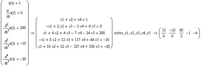
To evaluate the constants c1,c2,...,c5, in the general
solution in part A, we need to
1. Evaluate the solution x(t)
and its derivatives at t =0 and equate them to the initial
values.
2. Solve the resulting system for c1,c2,...,c5.
This will be done by creating a 5 x 1 vector containing
the solution and its derivatives evaluated at t = 0.
Mathcad will do the evaluations and gives 5 equations
in the unknowns c1,...,c5. Then the
solve command is used to solve the system.
Computer Project Two Solution
In this project, you will:
A. Use the help of Mathcad to find the general solution
of the fifth-order differential
equation
x(5)(t)
+ 3 x(4)(t)
+ 7 x(3)
(t) - 71 x''(t) + 24 x'(t) + 100 x(t) = 0
B. Use the initial conditions
x(0) = 1, x' (0) =0, x''(0) = 200,
x(3)(0)
= -10, x(4)(0)
= -20
to find a particular solution.
C. Use Mathcad's rkfixed
command to find an approximate solution of the differential
equation
D. Compare the exact solution in part (A) with the approximate
solution in part (B).
Part A
. (finding the general solution)
Step 1: Define the differential equation. The first
two terms of the differential equation are written
for you, add the rest of the terms
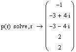
Step 2: Define the characteristic polynomial as p(r)
in terms of the variable r.
Step 3: Use the solve
command to find the roots of the characteristic polynomial.
Thus, with the computed values of c1, c2,....,c5 above,
the particular solution is:
To help you verify that your computation of the constants
c1, .. , c5 were correct, the solution and its derivatives
are evaluated at t = 0 below. They should return the
initial values. If any of the computed values does
not equal to the given initial value, then your computation
of the constants were incorrect.
Part C
. (finding a numerical solution)
In this part of the project you will use the
rkfixed command to
find a numerical solution (an approximate solution)
of the differential equation in part A over the interval
[

]
A vector setting the soluion and its derivatives
evaluated at t = 0 to the initial values
Result of the solve commad
Assign the computed values of c1,..., c5 to the variables
c1, c2, .. c5
Copy or retype your solution obtained in step 4 of part
A
(Do not delete. This is used to reset the value of t)