CHAPTER
SEVEN
Tests
of Hypotheses
7.1 Testing Hypotheses about a
Population Mean
Testing Hypotheses on the Mean
of a
Possible hypotheses, rejection region and probability values are summarized in the following table below.
Table 1 Testing hypotheses about a
population mean using z tests
|
|
Rejection Region |
|
|
|
|
|
|
|
|
|
|
|
|
|
where z is the test statistic, which can be
written
![]()
and
α is the significance level of the test.
Example 7.1
The average zinc concentration recovered from a
sample of zinc measurements in 36 different locations is found to be 2.6 grams
per millimeter. Assume that the population standard deviation is 0.3. It is
believed that the average zinc concentration of such measurements is less than
3 grams per millimeter. Set up suitable hypotheses and test at 1% level of
significance.
Solution From the sample we have ![]() . The hypotheses are given by
. The hypotheses are given by
![]()
The value of the test statistic z is given by
![]()
Since z = –8 < – zα = – 2.33 we
reject the null hypothesis ![]() , i.e. there is
sufficient evidence to reject the hypothesis that the mean zinc concentration
is 3.
, i.e. there is
sufficient evidence to reject the hypothesis that the mean zinc concentration
is 3.
Large Sample Test of the Population Mean
Refer
to Table 1 for the hypotheses. The test statistic is given by
![]()
Example 7.2 A
manufacturer of sports equipment has developed a new synthetic fishing line
that he claims has a mean breaking strength of 8 kilograms. At 1% level of
significance, test the hypothesis that the
mean breaking strength is 8 kilograms
against the alternative that mean breaking strength is not 8 kilograms if a
random sample of 50 lines is tested and found to have a mean breaking strength
of 7.8 kilograms and a standard deviation of 0.5 kilogram.
Solution The hypotheses are given by
![]()
The value of the test statistic z is given by

Since z = – 2.83 < – ![]() = – 2.575 we reject
= – 2.575 we reject ![]() and conclude that the
average breaking strength is not equal to 8.
and conclude that the
average breaking strength is not equal to 8.
Testing the Mean of a
Table 2 Testing hypotheses about a
population mean using t tests
|
|
Rejection Region |
p-value |
|
|
|
|
|
|
|
|
|
|
|
|
The test statistics t is given by
![]()
and ![]() is the
is the ![]() percentile of student t
distribution with
percentile of student t
distribution with ![]() degrees of freedom .
degrees of freedom .
Example 7.3 It is claimed that a vacuum
cleaner expends an average of 46 kilowatt-hours per year. If a random sample of
12 homes included in a planned study indicates that vacuum cleaners expend the
following kilowatt-hours per year
|
30 |
44 |
40 |
45 |
46 |
40 |
47 |
48 |
46 |
45 |
41 |
50 |
Does this suggest at the 5% level of significance
that vacuum cleaners expenses, on the average, is different from 46 kilowatt-hours annually?
Assume that the population of kilowatt-hours to be normal.
Solution The hypotheses are given by
![]()
The value of the test statistic t is given by

Since t = – 1.6447 is not less than ![]() , we can not reject the null hypothesis, i.e.
, we can not reject the null hypothesis, i.e. ![]() .
.
To solve the problem using Statistica, we follow the
steps:
1. Statistics
2. Basic
Statistics / Tables
3. T-test, single sample / OK
4. In T-test for
Single Means: Spreadsheet, Click Advanced to get Figure 7.1
5. Variables(
select the variable say Var1) / OK
6. In Reference
values input the value of ![]()
7. Summary
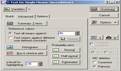
Figure 7.1 T-test for Single Means
These steps will give the
following results ( Figure 7.2):

Figure 7.2 Test of means against
reference constant (value)
Since the ![]() is too large compared
to
is too large compared
to ![]() , we cannot reject the null hypothesis at the5% level of
significance.
, we cannot reject the null hypothesis at the5% level of
significance.
7.2
Testing the Difference between Two Population Means
Testing the Difference between the Means of Two Independent
Table 3 Testing hypotheses about the
difference between the means of two
populations using z tests
|
|
Rejection Region |
|
|
|
|
|
|
|
|
|
|
|
|
|
Since
the assumption of known variances are not that realistic, we do not consider
any example here.
Large Sample Test of the Means of Two Independent Populations, Unknown
Variances
The test statistic z is given by
 .
.
Example 7.4 Consider
a tire manufacturer who wishes to estimate the difference between the mean
lives of two types of tires, Type A and Type B, as a prelude to a major
advertising campaign. A sample of 100 tires is taken from each production
process. The sample mean lifetimes are 30100 and 25200 miles respectively; the
sample variances are 1500000 and 2400000 miles squared respectively. Is there any difference between the mean
lives of the two types of tires at the 1% level of significance?
Solution: The hypotheses are given by
![]()
The value of the test statistic z is given by

Since z = 24.812 > ![]() = 2.575, we reject
= 2.575, we reject ![]() and accept
and accept ![]() .
.
Testing the Difference between the Means of Two Independent
Table 4 Testing hypotheses about the
difference between the means of two populations using t tests
|
|
Rejection Region |
|
|
|
|
|
|
|
|
|
|
|
|
|
The test statistic t is given by

with ![]() degrees of freedom and the pooled variance is given by
degrees of freedom and the pooled variance is given by
![]() .
.
Example
7.5 A random sample of
15 bulbs produced by an old machine was tested and found to have a mean life
span of 40 hours with standard deviation 5 hours. Also, a random sample of 10
bulbs produced by a new machine was found to have a mean life span of 45 hours
with standard deviation ![]() hours. Assume that the
life span of a bulb has a normal distribution for both machines, and true
variances are the same. Test at the 5% level of significance if there is any
difference between the mean lives of the bulbs produced by two machines.
hours. Assume that the
life span of a bulb has a normal distribution for both machines, and true
variances are the same. Test at the 5% level of significance if there is any
difference between the mean lives of the bulbs produced by two machines.
Solution The hypotheses are given by
![]()
Here, ![]()
![]()
![]() ,
, ![]()
![]()
![]() ,
, ![]() and
and ![]() . The estimate of common variance
. The estimate of common variance ![]() is
is ![]() The value of t given by
The value of t given by

Since t = –2.2625 < ![]() , we reject the null
hypothesis.
, we reject the null
hypothesis.
To solve the above problem using Statistica, the following steps can be used
1.
Statistics
2.
Basic
Statistics / Tables
3.
Difference
tests r, %, means / OK
4.
In
Difference between two mean (Normal distribution), input the values of M1, M2,
StDv1, StDv2, N1 and N2, then press Compute to get Figure 7.3.
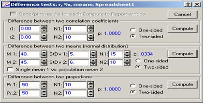
Figure 7.3 Difference
tests
The ![]() (See Figure 7.3)
provided by Difference Tests in Statistica is very much in agreement with what
we got by the probability calculator (in Statistica). Since the
(See Figure 7.3)
provided by Difference Tests in Statistica is very much in agreement with what
we got by the probability calculator (in Statistica). Since the ![]() , we reject the null hypothesis at the 5% level of
significance. Note that the option of one sided alternative hypotheses is
available in Statistica (See Figure 7.3).
, we reject the null hypothesis at the 5% level of
significance. Note that the option of one sided alternative hypotheses is
available in Statistica (See Figure 7.3).
Example
7.6 In order to compare two lifting
clubs, Club A and Club B, a sample of twenty weight liftings from the same
division were studied resulting in the data below:
|
Club
A |
251 251 |
247 254 |
249
259 |
251 250 |
249 252 |
250 256 |
254 243 |
245 251 |
257 242 |
249 248 |
|
Club
B |
249 250
|
251 249 |
259 251 |
248 250 |
259 253 |
252 257 |
249 249 |
251 253 |
251 249 |
253 251 |
We want to test the following
hypotheses:
![]() (the population means are identical)
(the population means are identical)
![]() (the population means are
not identical)
(the population means are
not identical)
The sample mean and variance for Club A are ![]() and
and ![]() , and the sample mean and variance for Club B are
, and the sample mean and variance for Club B are ![]() and
and ![]() . The pooled variance
. The pooled variance ![]() so that the value of test statistic is
so that the value of test statistic is ![]() , with
, with ![]()
Since
the observed ![]() = –1.0757 is not less than
= –1.0757 is not less than ![]() , we accept the null
hypothesis.
, we accept the null
hypothesis.
To
solve the above problem by Statistica, we need the following steps:
1. Enter each sample in a separate column
2. Statistics / Basic Statistics and Tables
3. t-test, independent, by variables (see
Figure 7.4) / OK
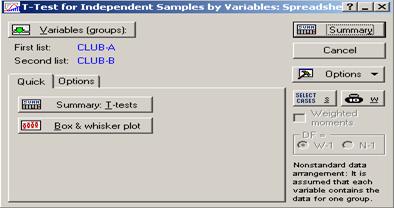
Figure 7.4 T-test for Independent
Variables
4. Click Variables [groups] and select
CLUB-A for first list and CLUB-B for second list / OK
5. In Quick click Summary: T-tests. These
steps give a scroll sheet of results (Figure 7.5).
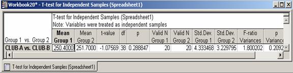
Figure 7.5 Results of t-test
Since
the ![]() , we cannot reject the null hypothesis at 5% level of
significance.
, we cannot reject the null hypothesis at 5% level of
significance.
Testing the Difference between the Means of Two Independent
Refer to Table 4 for hypotheses. The value of the
test statistic t is given by

with ![]() degrees of freedom.
degrees of freedom.
Example 7.7 A
random sample of 16 bulbs produced by an old machine was tested and found to
have a mean life span of 40 hours with standard deviation 5 hours. Also,
another random sample of 16 bulbs produced by a new machine was found to have a
mean life span of 45 hours with standard deviation 6 hours. Assume that the
life span of a bulb has a normal distribution for both machines, test at the1%
level of significance if the mean life of the bulbs produced by the new machine
is more than that by the old machine.
Solution The hypotheses to be tested
are given by
![]()
Since there is no information about the equality of
variances but the sample sizes are the same we would go for the simpler test
given by

with ![]() df. With
df. With ![]() , since t = –2.561 <
, since t = –2.561 < ![]() , we reject the null hypothesis.
, we reject the null hypothesis.
Testing the Difference between Means of Two Normal Populations, Neither
the Variances nor the Sample Sizes are Equal
Refer to Table 4 for the hypotheses testing. The
value of the test statistic t is given by

with degrees of freedom 
Example 7.8 A
random sample of 12 bulbs produced by an old machine was tested and found to
have a mean life span of 40 hours with variance 24 hours. Also, a random sample
of 10 bulbs produced by a new machine was found to have a life span of 45 hours
with variance 30 hours. Assume that the life span of a bulb has a normal
distribution for both machines, and but the true variances are not the same.
Test at the 5% level of significance if there is any difference between the
mean lives of the bulbs produced by two machines.
Solution The
hypotheses to be tested are given by
![]() .
.
For old machine, we have ![]() and for new machine,
we have
and for new machine,
we have![]() . The degrees of freedom is
. The degrees of freedom is ![]() and the test statistic is
and the test statistic is ![]() . Since
. Since ![]() <
< ![]() , we reject the null
hypothesis at the 5% level of significance.
, we reject the null
hypothesis at the 5% level of significance.
Testing
the Difference between Two Population Means; Matched Pairs Case
Refer to Table 4 for the hypotheses. The test statistic t is given by
![]()
where ![]() is the mean of the
differences between the paired observations, and
is the mean of the
differences between the paired observations, and ![]() is the corresponding standard deviation, and the number of degrees of freedom is
is the corresponding standard deviation, and the number of degrees of freedom is ![]() .
.
Example 7.9
For the data in Example 6.9, test at 5% level of significance if there is
any difference in mean time by CAD and by Traditional Method.
Solution We want to test the
hypotheses that
![]()
The value of the test statistic is
![]()
With ![]() and
and ![]() ,
, ![]() . Since
. Since ![]() is not less than
is not less than ![]() , we do not reject the null hypothesis.
, we do not reject the null hypothesis.
The
above problem can be solved using Statistica following the steps:
- Enter each sample in a
separate column
- Statistics / Basic
Statistics and Tables
- t-test, Dependent
sample (see Figure 7.6) / Ok
- Variables (First list
and Second list) / OK
- In Quick: click Summary:
T-test
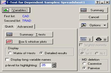
Figure 7.6 T-test for Dependent Samples
Since the ![]() (See Figure 7.7), we
reject the null hypothesis at
(See Figure 7.7), we
reject the null hypothesis at ![]() (in fact for any
(in fact for any ![]() but accept at
but accept at ![]() (in fact for any
(in fact for any![]() ). Note that many statisticians support keeping
). Note that many statisticians support keeping ![]() at a low level not
exceeding 5%.
at a low level not
exceeding 5%.
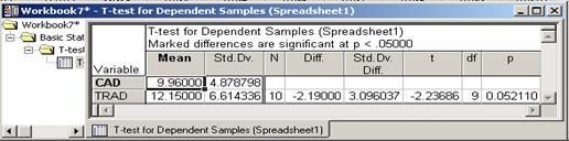
Figure 7.7 Spreadsheet for t-test
(Dependent Samples)
7.3 Large Sample Tests of Proportions
Testing a Population
Proportion
Tests on ![]() are summarized in the
following table:
are summarized in the
following table:
Table 5 Testing hypotheses for the
population proportion
|
|
Rejection Region |
|
|
|
|
|
|
|
|
|
|
|
|
|
The test statistics z is given by
 .
.
Example 7.10 In certain water-quality
studies, it is important to check for the presence or absence of various types
of microorganisms. Suppose 20 out of 100 randomly selected samples of a fixed
volume show the presence of a particular microorganism. At the 1% level of significance, test the
hypothesis that the true proportion of the presence of a particular
microorganism is at least 0.30.
Solution The hypotheses are given by
![]() .
.
with ![]() , the Rejection Region is given by. Since the observed
, the Rejection Region is given by. Since the observed
![]()
Since z = –2.18 is
not less than ![]() = 2.33, we accept the
null hypothesis.
= 2.33, we accept the
null hypothesis.
Large Sample Test
of the Difference between Two Population Proportions
Table 6 Testing hypotheses about the
difference between two population proportions
|
|
Rejection Region |
|
|
|
|
|
|
|
|
|
|
|
|
|
where the test statistic z is given by
 , where
 ![]()
Note
that ![]() is the number of items in the sample from Population I having
a particular characteristic, and
is the number of items in the sample from Population I having
a particular characteristic, and![]() is the number of items in the sample from Population II
having a particular characteristic
is the number of items in the sample from Population II
having a particular characteristic
Example
7.11 The fraction defective product produced by
two production lines is being
analyzed. A random sample of 1000 units from Line I has 10 defectives, while a
random sample of 1200 units from Line II has 25 defectives. Is there any
significant difference between the fraction defectives of the two production
lines? (Assume that ![]() )
)
Solution The hypotheses are given by
![]() .
.
Here
![]()
![]() . The value of the test statistic is given by
. The value of the test statistic is given by
 .
.
Since z = –2.0221 is not less than ![]() , we accept the null hypothesis, and conclude that the
evidence does not support the difference.
, we accept the null hypothesis, and conclude that the
evidence does not support the difference.
To solve the above
problem by using Statistica, we need to the following steps
1.
Statistics
2.
Basic
Statistics / Tables
3.
Difference
tests r, %, means / OK to get Figure 7.8
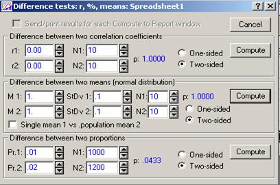
Figure 7.8 Difference
tests
We put ![]() for Pr.1 and
for Pr.1 and ![]() for Pr.2 in Figure 7.8.
Since the
for Pr.2 in Figure 7.8.
Since the![]() , we reject the null hypothesis at 5% level of significance.
, we reject the null hypothesis at 5% level of significance.
Exercises
7.1
(cf.
Johnson, R. A., 2000, 126). The following random samples are measurements of the
heat-producing capacity (in millions of calories per ton) of specimens of coal
from two mines:
|
Mine
1 |
8260 |
8130 |
8350 |
8070 |
8340 |
7990 |
|
Mine
2 |
7950 |
7890 |
7900 |
8140 |
7920 |
7840 |
(a) Use the 0.01
level of significance to test whether the difference between the means of these
two samples is significant, assuming equal variances.
(b) Repeat part
(a) (assuming unequal variances).
7.2
(Johnson,
R. A., 2000, 264). The following are the average weekly losses of worker-hours due to
accidents in 10 industrial plants before and after a certain safety program was
put into operation:
|
Before
|
45 |
73 |
46 |
124 |
33 |
57 |
83 |
34 |
26 |
17 |
|
After |
36 |
60 |
44 |
119 |
35 |
51 |
77 |
29 |
24 |
11 |
Use the 0.05 level of significance to test whether
the safety program is effective.
7.3
(cf.
Johnson, R. A., 2000, 266). As part of an industrial training program, some
trainees are instructed by Method A, which is straight teaching machine
instruction and some are instructed by Method B, which also involve the
personal attention of an instructor. If random samples of size 10 are taken
from large group of trainees instructed by each of these two methods, and the
scores which they obtained in an appropriate achievement test are
|
Method
A |
71 |
75 |
65 |
69 |
73 |
66 |
68 |
71 |
74 |
68 |
|
Method
B |
72 |
77 |
84 |
78 |
69 |
70 |
77 |
73 |
65 |
75 |
(a) Use the 0.05
level of significance to test the claim that both the methods have same
results. Assume that ![]() .
.
(b) Use the 0.05
level of significance to test the claim that both the methods have same
results. Assume that ![]() .
.
7.4
(cf.
Johnson, R. A., 2000, 266). The following are the number of sales which a sample
of 9 salespeople of industrial chemicals in
|
|
59 |
68 |
44 |
71 |
63 |
46 |
69 |
54 |
48 |
|
|
50 |
36 |
62 |
52 |
70 |
41 |
58 |
39 |
60 |
Test the null hypothesis ![]() = 0 against the alternative hypothesis
= 0 against the alternative hypothesis ![]()
![]() 0 at the 0.01 level of significance.
0 at the 0.01 level of significance.
7.5
(Johnson,
R. A., 2000, 266). The following are the Brinell hardness values obtained by samples of
two magnesium alloys:
|
Alloy
1 |
66.3 |
63.5 |
64.9 |
61.8 |
64.3 |
64.7 |
65.1 |
64.5 |
68.4 |
63.2 |
|
Alloy
2 |
71.3 |
60.4 |
62.4 |
63.9 |
68.8 |
70.1 |
64.8 |
68.9 |
65.8 |
66.2 |
Use the 0.05 level of significance to test the null
hypothesis ![]() = 0 against the alternative hypothesis
= 0 against the alternative hypothesis ![]()
![]() 0.
0.
7.6
(Johnson,
R. A., 2000, 267). To compare two kinds of bumper guards, 6 of each kind were mounted on a
certain kind of compact car. Then each car was run into a concrete wall at 5
miles per hour, and the following are the costs of the repairs (in dollars):
|
Bumper
Guard 1 |
107 |
148 |
123 |
165 |
102 |
119 |
|
Bumper
Guard 2 |
134 |
125 |
112 |
151 |
133 |
129 |
Use the 0.01 level of
significance to test whether there is a difference between the two population
means.
7.7
(Johnson,
R. A., 2000, 267). The following data were obtained in an experiment designed to check
whether there is a systematic difference in the weights obtained with two
different scales:
|
Rock |
1 |
2 |
3 |
4 |
5 |
6 |
7 |
8 |
9 |
10 |
|
Scale 1 |
11.23 |
14.36 |
8.33 |
10.50 |
23.42 |
9.15 |
13.47 |
6.47 |
12.40 |
19.38 |
|
Scale 2 |
11.27 |
14.41 |
8.35 |
10.52 |
23.41 |
9.17 |
13.52 |
6.46 |
12.45 |
19.35 |
Use the 0.05 level of
significance to test whether the difference of the weights obtained with the
two scales is significant.
7.8
(cf.
Montgomery, D. C., et. al, 2001, 229). Two catalysts are being analyzed to determine
how they affect the mean yield of a chemical process. A test is run in the
pilot plant and results are;
|
Catalyst
1 |
91.50 |
94.18 |
92.18 |
95.39 |
91.79 |
89.07 |
94.72 |
89.21 |
|
Catalyst
2 |
89.19 |
90.95 |
90.46 |
93.21 |
97.19 |
97.04 |
91.07 |
92.75 |
Is
there any difference between the mean yields? Use a = 0.05.
(a) Assuming equal
population variances.
(b) Assuming
unequal population variances.
7.9
(Johnson,
R. A., 2000, 267). In a study of the effectiveness of physical exercise in weight reduction,
a group of 14 persons engaged in a prescribed program of physical exercise for
one month showed the following results:
|
Weights
before (Ibs) |
209 |
178 |
169 |
212 |
180 |
192 |
180 |
|
196 |
171 |
170 |
207 |
177 |
190 |
180 |
|
|
Weights
after (Ibs) |
170 |
153 |
183 |
165 |
201 |
179 |
144 |
|
164 |
152 |
179 |
162 |
199 |
173 |
140 |
Use the 0.01 level of
significance to test whether the prescribed program of exercise is effective.
Montgomery, Runger and Hubele (2001).
7.10
(cf.
|
M1 |
16.03 |
16.04 |
16.05 |
16.05 |
16.02 |
16.01 |
15.96 |
15.98 |
16.02 |
15.99 |
|
M2 |
16.02 |
15.97 |
15.96 |
16.01 |
15.99 |
16.03 |
16.04 |
16.02 |
16.01 |
16.00 |
(a) Do you think
the engineer is correct? Use a= 0.05. Use![]()
(b) What is the
probability value for this test?
(c) Do you think
the engineer is correct? Use a= 0.05.![]()
7.11
(cf.
Montgomery, D. C., et. al, 2001, 238). The deflection temperature under load for two
different types of plastic pipe is being investigated. Two random sample of 15
pipe specimen are tested and the deflection temperatures observed are reported
here (in ![]() F).
F).
|
Type
1 |
206 |
188 |
205 |
187 |
194 |
193 |
207 |
205 |
|
185 |
189 |
213 |
192 |
210 |
194 |
178 |
192 |
|
|
Type
2 |
177 |
197 |
206 |
201 |
180 |
176 |
185 |
195 |
|
200 |
197 |
192 |
198 |
188 |
189 |
203 |
192 |
(a) Do the data
support the claim that the deflection temperature under load for both types is
same? Use a = 0.05
(b) Calculate the
probability value for the test in part (a).
7.12
(cf.
Montgomery, D. C., et. al, 2001, 239). In semiconductor manufacturing, wet chemical
etching is often is used to remove silicon from the backs of wafers prior to
metalization. The etch rate is an important characteristic in this process and
known to follow a normal distribution. Two different etching solutions have
been compared, using two random samples of 10 wafers from each solution. The
observed etch rates are as follows (in mils/min):
|
Solution
1 |
9.9 |
9.4 |
9.3 |
9.6 |
10.2 |
10.6 |
10.3 |
10.0 |
10.3 |
10.1 |
|
Solution
2 |
10.2 |
10.6 |
10.7 |
10.4 |
10.5 |
10.0 |
10.2 |
10.7 |
10.4 |
10.3 |
Do the data support the
claim that the mean etch rate is same for both the solutions? Use a = 0.05
(a) Assume ![]() .
.
(b) Assume![]() .
.
(c) Calculate the ![]() for the test in part
(a).
for the test in part
(a).
7.13 Refer to Exercise 6.7, Conduct the most appropriate
hypothesis test using a 0.05 significance level
7.14 Refer to Exercise 6.8, Conduct the most appropriate
hypothesis test using a 0.01 significance level
7.15 Refer to Exercise 6.9, Conduct the most appropriate
hypothesis test using a 0.01 significance level.
7.16 Refer to Exercise 6.10, Conduct the most appropriate hypothesis test
using a .01 significance level.
7.17 Refer to Exercise 6.11, Conduct the most appropriate hypothesis test
using a 1% significance level
7.18 Refer to Exercise 6.12, Conduct the most appropriate hypothesis test
using a 0.05 significance level.
7.19 Refer to Exercise 6.13, Conduct the most appropriate hypothesis
test using a .01 significance level.
7.20 Refer to Exercise 6.14, Conduct the most appropriate hypothesis
test using a .01 significance level.
7.21 Refer to
Exercise 6.15, Conduct
the most appropriate hypothesis test using a 0.05 significance level.
7.22 Refer to
Exercise 6.16, Conduct
the most appropriate hypothesis test using a 0.05 significance level.
7.23 Refer
to Exercise 6.17,
Conduct the most appropriate hypothesis test using a 0.05 significance level.
7.24 Refer to Exercise 6.18, Conduct
the most appropriate hypothesis test using a .05 significance level.
7.25 Refer to Exercise 6.22, Conduct
the appropriate hypothesis test using a 0.05 significance level.
7.26 Refer to Exercise
6.23, Conduct the appropriate hypothesis test using a 0.10 significance level.
7.27 Refer to
Exercise 6.24, Conduct the appropriate hypothesis test using a .05 significance
level.
7.28 Refer to
Exercise 6.25, Conduct the appropriate hypothesis test using a 0.01
significance level.
7.29 Refer to
Exercise 6.26, Conduct the appropriate hypothesis test using a 0.05
significance level.
7.30 Refer to
Exercise 6.27, Conduct
the appropriate hypothesis test using a 0.10 significance level