Section 11.5 Inferences Concerning the Regression Coefficients

Example 11.2. 1

Example 11.3. 2

Minitab Example: 2

Example 11.4. 3

Example 11.5. 3

Example 11.6. 5

Example 11.7. 6

Example 11.10. 10

Example 11.11. 11

Example 11.12. 11

Important: 12

Confidence Interval for b , the slope parameter

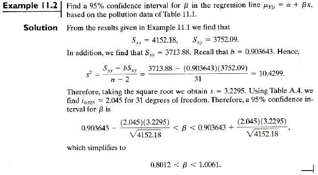
A (1-a)100% confidence interval for the parameter b in the regression line m_Y|x = a + bx is

where is a value of the t-distribution with n-2 degrees of freedom

Example 11.2

Hypothesis testing on the slope parameter, b

To test the null hypothesis H_o:b = b_o against any suitable alternatives,

use t-distribution with n-2 degrees of freedom to define the critical region, and the following test statistic

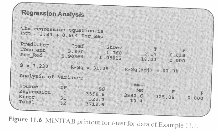
Example 11.3

Minitab Example:

Statistical Inference on the intercept

Confidence Interval for a , the intercept parameter

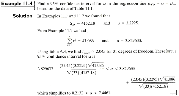
A (1-a)100% confidence interval for the parameter a in the regression line m_Y|x = a + bx is

or

where is a value of the t-distribution with n-2 degrees of freedom

Example 11.4

Hypothesis testing on the intercept parameter, a

To test the null hypothesis H_o: a = a_o against any suitable alternatives,

use t-distribution with n-2 degrees of freedom to define the critical region, and the following test statistic

Example 11.5

df=33-2=31, P-value =

From Table A.4 directly, P-value < 0.05. So, the null hypothesis of zero intercept is rejected at 0.05 level of significance.

A measure of quality of fit: Coefficient of Determination, R²

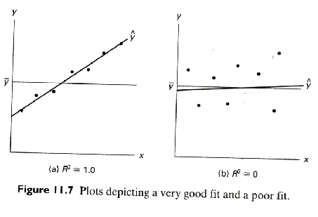
Coefficient of Determination, R² = proportion of total variability in the dependent variable Y explained by the fitted model.

TSS = SSR + SSE

Coefficient of Determination,

R² = 1.0 if fit is perfect

R² = 0.0 if fit is poor

Section 11.6 Prediction

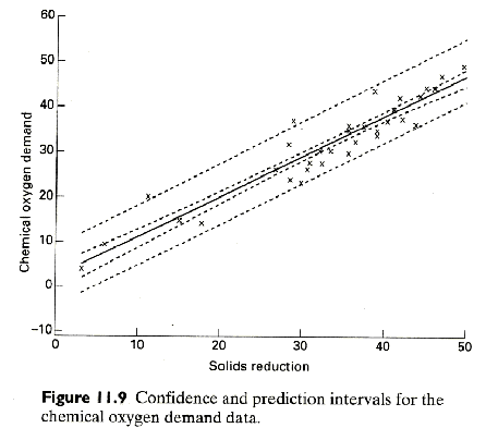
Confidence Interval for , the mean response

A (1-a)100% confidence interval for the mean response in the regression line m_Y|x = a + bx is

where is a value of the t-distribution with n-2 degrees of freedom

Example 11.6

Prediction Interval for , the future value of a response

A (1-a)100% prediction interval for a single response in the regression line m_Y|x = a + bx is

where is a value of the t-distribution with n-2 degrees of freedom

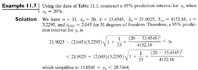
Example 11.7

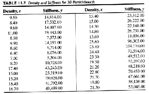
Section 11.11 Simple Linear Regression Case Study

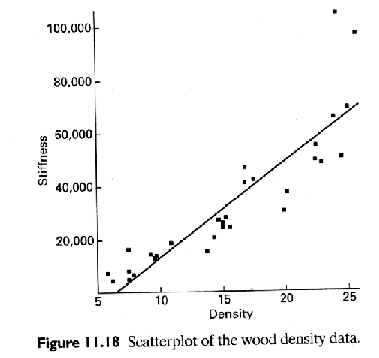
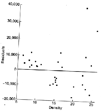
A more complicated model may be more appropriate

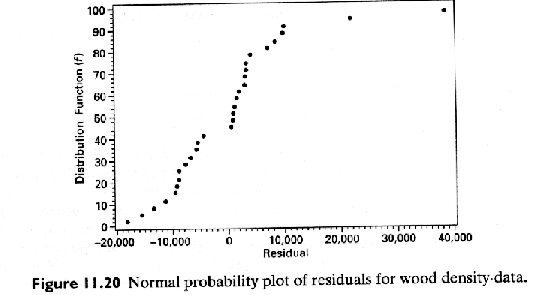
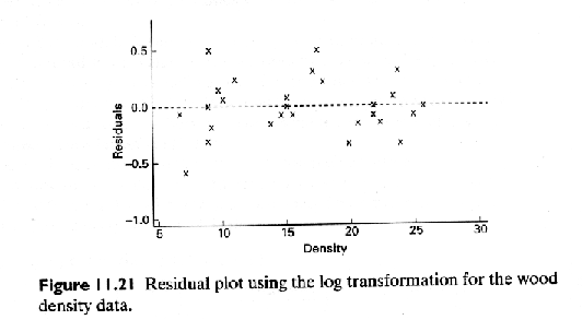
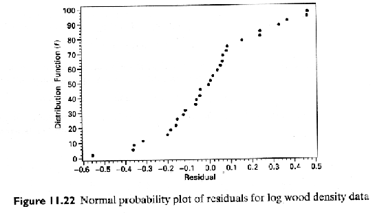
The higher R² value would suggest that the transformed model is more appropriate.

Section 11.12 Correlation

Correlation coefficient

The measure r of linear association between two variables X and Y is estimated by the sample correlation coefficient r, where

-1 < r < 1

r = 1.0 or –1.0 perfect linear relationship

r = 0.0 no linear relationship

Sample coefficient of determination

represents the proportion of the variation in TSS explained by the regression of Y on x, namely, SSR.

Example 11.10

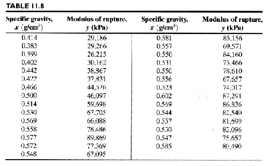
Hypothesis testing on the correlation coefficient, r

To test the null hypothesis H_o: r = r_o against any suitable alternatives,

We can use t-distribution with n-2 degrees of freedom to define the critical region, and the following test statistic

but this test has problem when r values close to -1 or 1

However, a more general test is given by

the approximate normal distribution with mean and variance .

We can use the standard normal to define the critical region, and the following test statistic

Example 11.11

Example 11.12

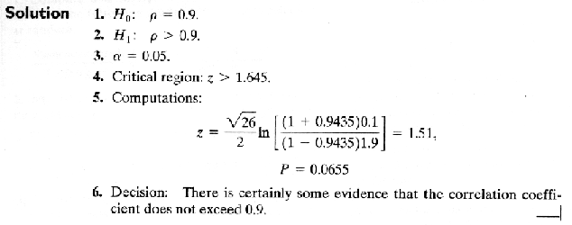
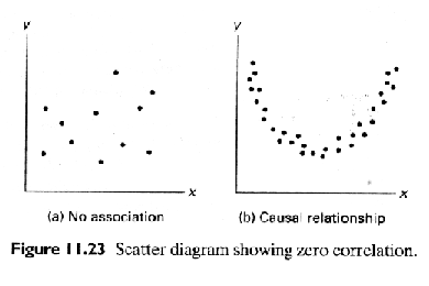
Important: Correlation is a measure of linear relationship, so r = 0 does not necessarily mean there is no relationship between two variables.