CHAPTER
FOUR
Continuous Random Variables
The following table contains some of
the most well known, and often used continuous distributions in Engineering.
Table 1 Some Continuous Random Variables and
Their Means and Variances
|
Distribution |
Density Function |
Mean |
Variance |
|
Exponential |
|
|
|
|
|
|
|
|
|
Gamma |
|
|
|
|
Weibull |
|
|
|
|
Lognormal |
|
|
|
|
Beta |
|
|
|


4.1 The Probability Calculator
The probability
calculator can be used to compute probabilities for continuous random
variables. It is accessed through the Basic Statistics and tables module following
the steps:
(1) Statistics/ Basic
Statistics and Tables (getting Figure 4.1)
(2) Probability
Calculator
(3) OK.
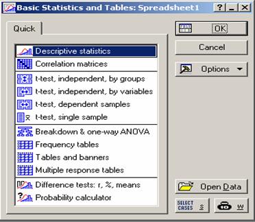
Figure 4.1 Basic Statistics and Tables: Spreadsheet
By default, this opens the probability distribution calculator
menu for the Beta random variable with shape parameters 2 and 2 as shown in
Figure 4.2.
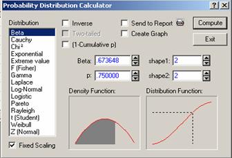
Figure 4.2 Probability Distribution Calculator
To compute the probability for a particular continuous
random variable, its distribution is highlighted and the appropriate parameters
are supplied. It is helpful to view the
graph of the density function as it gives visual insight of the type of
probability function under consideration. Note that for continuous random
variables, the probability is represented by the area under the probability
density function. In case the density function is invisible, uncheck Fixed Scaling (see the bottom left corner of Figure 4.2).
The Inverse,
Two-tailed and (1-Cumulative
p) functions are available for calculation of the probability
of an event or calculation of a quartile. While using the probability
calculator, it is important to view the shaded part of the graph of the density
function and make sure that the shaded part corresponds to the event of interest.
4.2 The Exponential Distribution
Example 4.1 Life length of a particular type of battery follows
exponential distribution with mean 2 hundred hours. Find the probability that
the
(a) life length of a particular battery of this
type is less than 2 hundred hours.
(b) life length of a particular battery of this
type is more than 4 hundred hours.
(c) life length of a particular battery of this
type is less than 2 hundred hours or more
than 4 hundred hours.
Solution Let ![]() = life length of a battery. Then
= life length of a battery. Then![]() , by
, by ![]() (given) so that
(given) so that ![]()
(a)
![]()
(b)
![]()
(c)
![]()
Computing Exponential Probabilities Using Statistica
To
compute the probability of an event related to the exponential random variable,
select Exponential from the distribution list of the Probability
Distribution Calculator (see Figure 4.3), next supply lambda,
and the value of x in the
exp. slot.
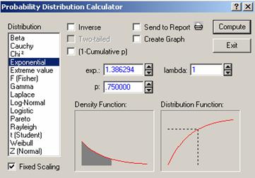
Figure 4.3 Exponential probability calculator
In the Exponential probability calculator,
we have the following two cases:
Case 1: Leaving the Inverse and (1-
cumulative p) unchecked
If the Inverse and (1-cumulative p) functions are unchecked, a figure similar to Figure
4.3 is obtained for the exponential random variable. The shaded area under the
density function indicates a probability of the form P(X < u) = p where u
= 1.386294 is the value of X, l = 1 and p = 0.75. That is, Figure 4.3 shows that P(X < 1.386294) = 0.75 where X is an exponential random variable with
parameter l = 1.
So to
compute the probability that the exponential random variable is less than or
equal to 2 in part (a) in Example 4.1, enter 2 for the value of x in the exp. slot and enter 0.5 for lambda and then click Compute
to read the probability value in the slot for
p.
To find
u such that P(X < u) = 0.82 where the
random variable X has an exponential
distribution with parameter l = 3,
put 0.82 for p, 3 for lambda, and
click compute to get u = 0.571599
which is
in the exp. slot. Gradually we will be using the notation u = 0.571599 = ![]() meaning that
meaning that ![]() and
and ![]() .
.
Case
2: (1-Cumulative p) checked
When
(1-Cumulative p) is checked for the exponential random
variable as shown in Figure 4.4, we obtain a probability of the form P(X
> u). To find P(X > 4) where X has an exponential distribution with
parameter 2, check (1-Cumulative p), put 2 for lambda and 4 for X in the exp. slot, then click compute, to get p = 0.000335, i.e., P(X
> 4) = 0.000335 (Figure 4.4).
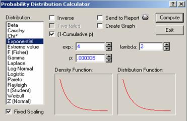
Figure 4.4 Checking (1-Cumulative p) only
It is
possible to find ![]() such that
such that ![]() where
where ![]() has an exponential distribution with parameter
has an exponential distribution with parameter![]() . Check (1-Cumulative
p), put 0.75 for
. Check (1-Cumulative
p), put 0.75 for ![]() and 3
for lambda,
click “Compute” to get the value of
and 3
for lambda,
click “Compute” to get the value of ![]() in the exp. Slot, i.e,
in the exp. Slot, i.e, ![]()
![]()
![]() , which is the 25th percentile of exponential
distribution with parameter 3.
, which is the 25th percentile of exponential
distribution with parameter 3.
4.3 The Normal Distribution
When
the mean of a normal distribution equals 0, and the variance equals 1, we get
what we call a standard normal random Z. Its density is given by
![]()
Computing Standard
Using the standard normal probability table in Appendix
A2 we can find the following:
P(Z < 2.13) = 0.9834
P(Z > –1.68) = 0.9535
P(–1.02 < Z < 1.51) = 0.9345 – 0.1562 = 0.7783
Computing
Example 4.2 A manufacturing process has a machine that fills
coke to 300 ml bottles. Over a long period of time, the average amount
dispensed into the bottles is 300 ml, but there is a standard deviation of 5 ml
in this measurement. If the amounts of fill per bottle can be assumed to be
normally distributed, find the probability that the machine will dispense
between 295 and 310 ml of liquid in any one bottle. (cf. Scheaffer and McClave,
1995, 216-217).
Solution Let ![]() = amount of fill in a bottle. Then
= amount of fill in a bottle. Then ![]()

Example 4.3 The compressive strength of
samples of cement can be modeled by a normal distribution with a mean of 6000
kilograms per square centimeter and a standard deviation of 100 kilograms per
square meter.
(a) What is the probability that the strength of
a sample is less than 6164.5 kg/cm![]() ?
?
(b) What compressive strength is exceeded by 95%
of the time?
(c) What compressive strength exceeds 5% of the
time?
Solution (a) ![]()
(b) ![]()
From
the Standard Normal Probability Table, ![]() so that by comparison
we have
so that by comparison
we have ![]() .
.
Computing Standard
To compute probabilities for a standard normal random
variable, select Z(
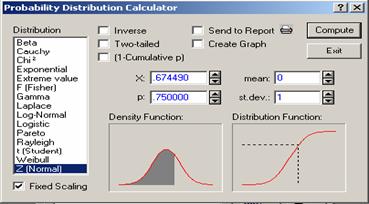
Figure 4.5 The Z (
Case 1: Leaving
the Inverse, Two-tailed and (1- Cumulative
p) unchecked
The
default option is![]() . To calculate
. To calculate![]() , put 0.67449 (=a) for
, put 0.67449 (=a) for ![]() and click “compute” to
get the required probability to be 0.75, that is,
and click “compute” to
get the required probability to be 0.75, that is, ![]() as in Figure 4.5. The quantity
as in Figure 4.5. The quantity ![]() in the figure is the value of the standard normal random
variable
in the figure is the value of the standard normal random
variable![]() .
.
To
calculate the 75th percentile i.e. to find ![]() such that
such that ![]() enter 0.75 for
enter 0.75 for ![]() and click “compute” to get 0.67449 i.e.
and click “compute” to get 0.67449 i.e. ![]() meaning a = 0.67449 =
meaning a = 0.67449 = ![]() , the 75th percentile or the third quartile of the
standard normal random variable.
, the 75th percentile or the third quartile of the
standard normal random variable.
Case 2: Only Two-tailed checked
Check
only Two-tailed to
calculate a probability of the form ![]() . For example, to
calculate
. For example, to
calculate ![]() put 1.439531 for
put 1.439531 for ![]() and click “compute” to
get 0.85 under p,
see Figure 4.6.
and click “compute” to
get 0.85 under p,
see Figure 4.6.
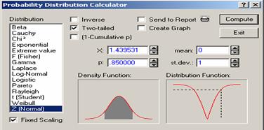
Figure 4.6 Only Two-tailed Checked
Case 3: Only (1-Cumulative p) checked
To
evaluate ![]() click (1-Cumulative p), put 1.439531 for x and click “compute” to get 0.075, i.e.
click (1-Cumulative p), put 1.439531 for x and click “compute” to get 0.075, i.e. ![]() (see Figure 4.7).
(see Figure 4.7).
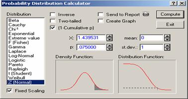
Figure 4.7 Only (1-cumulative
p) Checked
Let ![]() denote the
denote the ![]() percentile of Standard
Normal Distribution. For example
percentile of Standard
Normal Distribution. For example ![]() or equivalently
or equivalently![]()
Thus, ![]() , which is the 97.5th percentile of the Standard
Normal Distribution. You can check that
the quartiles of the distribution are given by
, which is the 97.5th percentile of the Standard
Normal Distribution. You can check that
the quartiles of the distribution are given by ![]() and
and ![]() .
.
To find the 92.5th
percentile, i.e. to find ![]() such that
such that ![]() = 0.075, check (1-Cumulative
p), put 0.075 for
= 0.075, check (1-Cumulative
p), put 0.075 for ![]() and click “compute” to
get 1.439531, i.e.
and click “compute” to
get 1.439531, i.e. ![]() = 0.075 (see
Figure 4.7).
= 0.075 (see
Figure 4.7).
Case 4: Two-tailed and (1- Cumulative p) checked
If both the Two-tailed and (1-Cumulative p)
are checked for the standard normal random variable, then the probability being
computed is of the form
![]() .
.
Thus, to calculate ![]() , check both Two-tailed
and (1-Cumulative p)
function put 1.439531 for x and click
“compute” to get 0.15. i.e.
, check both Two-tailed
and (1-Cumulative p)
function put 1.439531 for x and click
“compute” to get 0.15. i.e. ![]() =
= ![]() = 0.15. (See
Figure 4.8).
= 0.15. (See
Figure 4.8).
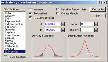
Figure 4.8 Two-tailed and (1-Cumulative p) Checked
Case 5: Two-tailed and Inverse checked
Similarly, one can obtain the value of a, such that ![]() by checking both the Two-tailed and Inverse, and putting 0.15 for p.
The solution to a is 1.439531 in the
slot for x.
by checking both the Two-tailed and Inverse, and putting 0.15 for p.
The solution to a is 1.439531 in the
slot for x.
Finding
the Values ![]() and
and ![]() of the Standard
of the Standard
The
value of the standard random variable for which the probability is a to its right is denoted by za and a is called the tail probability. For instance, if we have ![]() , then the value 1.439531 has a probability of 0.075 to its
right, i.e.,
, then the value 1.439531 has a probability of 0.075 to its
right, i.e., ![]() (see Case 3 and Figure
4.7 above).
(see Case 3 and Figure
4.7 above).
![]() is the value of the standard
random variable having probability (or an area) of
is the value of the standard
random variable having probability (or an area) of ![]() to its right. Given
the value of a, we may find the value of
to its right. Given
the value of a, we may find the value of ![]() by checking the Two-tailed and (1-Cumulative p) together, and entering a for p in the standard normal
probability calculator. The value computed for x is then read as the za/2 value. For example, in
Figure 4.8, za/2 is computed in x as 1.439531, where
by checking the Two-tailed and (1-Cumulative p) together, and entering a for p in the standard normal
probability calculator. The value computed for x is then read as the za/2 value. For example, in
Figure 4.8, za/2 is computed in x as 1.439531, where ![]() . This provides
. This provides ![]()
Alternatively, the value of ![]() may be found by first finding a/2 and using it for p as in Case 3 (see Figure 4.7).
may be found by first finding a/2 and using it for p as in Case 3 (see Figure 4.7).
Probabilities of
All the illustrations have
been done so far using the standard normal random variable. In the case of normal random variables, the
principle remains the same, but care needs to be taken in the interpretation of
the two-tailed
probabilities.
Case 1: Leaving the Inverse, Two-tailed and 1-Cumulative p unchecked
To calculate ![]() where
where ![]() with
with ![]()
![]() and
and ![]() say, put 60 for mean, 25 for standard deviation and 90 for '
say, put 60 for mean, 25 for standard deviation and 90 for '![]() '. Beware that '
'. Beware that '![]() ' in Figure 4.9 is the value '
' in Figure 4.9 is the value '![]() ' of random variable X.
' of random variable X.
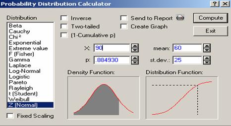
Figure 4.9 Normal Distribution with Inverse, Two-tailed and
(1-Cumulative p) unchecked
Case 2:
To calculate ![]() click Two-tailed and proceed, for example to calculate
click Two-tailed and proceed, for example to calculate ![]() where X
is a normal random variable with
where X
is a normal random variable with ![]() enter 60 for mean, 30 for standard deviation and 90 for x. This provides
0.769861 for p, i.e.,
enter 60 for mean, 30 for standard deviation and 90 for x. This provides
0.769861 for p, i.e., ![]() , see Figure 4.10. Note
that if the interval (a, b) is not symmetric about
the mean, then compute
, see Figure 4.10. Note
that if the interval (a, b) is not symmetric about
the mean, then compute ![]() as
as ![]() .
.
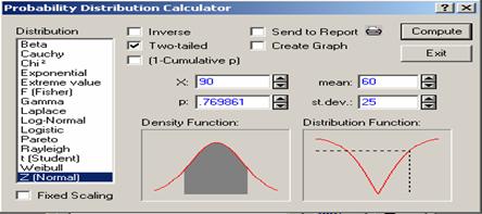
Figure 4.10 Normal Distribution with only Two-tailed Checked
Case 3:
Figure
4.11 shows the probability calculator for the normal variable having the mean
of 60 and standard deviation of 25 with both Two-tailed
and (1-Cumulative p) checked. To calculate ![]() chick both Two-tailed
and (1-Cumulative p). Let
chick both Two-tailed
and (1-Cumulative p). Let
![]()
![]() and
and ![]() . To calculate
. To calculate ![]() =
= ![]() +
+ ![]() put 90 for x to get 0.230139 for p,
i.e.,
put 90 for x to get 0.230139 for p,
i.e., ![]()
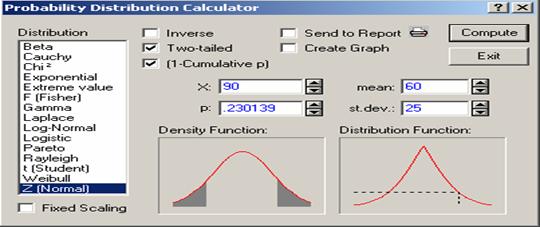
Figure 4.11 Normal distribution with Two-tailed
and (1-cumulative p) Checked
4.4
Other Distributions
The
Gamma Probability Calculator
The
probability density function of the gamma random variable is given by
![]()
The
Gamma probability calculator provides probability of events of
the type X < a for the Gamma distribution with shape parameter a.
To calculate P(X< 1.386294), where X has Gamma distribution with shape parameter a = 1, put 1.386294 for G (the value of X) and 1 for shape, then click “compute” to get 0.75 for p, i.e. P(X< 1.386294) = 0.75 (see Figure 4.12).
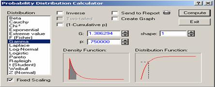
Figure 4.12 Probability Calculator for the
Gamma Distribution
Similarly, to calculate P(X< 1.386294), where X has a Gamma distribution with a = 2, put 2 for the shape and 1.386294 for G and click “compute” to get 0.403426 for p, i.e., P(X< 1.386294) = 0.403426.
The
Weibull Probability Calculator
The
Weibull Probability calculator provides the probability of events of the type W < a for scale parameter b and shape parameter a of Weibull distribution. Plots of the probability
density function and cumulative distribution function are also available.
To calculate ![]() put 1.386294 for w,
1 for shape and 1 for scale, then click “compute” to
get 0.75 for
put 1.386294 for w,
1 for shape and 1 for scale, then click “compute” to
get 0.75 for ![]() , i.e.
, i.e. ![]() (see Figure 4.13).
(see Figure 4.13).
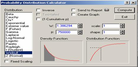
Figure 4.13 Probability Calculator for the
Weibull Distribution
Similarly,
for the Weibull distribution with scale parameter ![]() and shape parameter
and shape parameter ![]() , one can calculate
, one can calculate ![]() by putting 2 for the shape, 3 for the scale and 1.386294 for w (which is the value of W)
and click “compute” to get 0.192276 for p, i.e.,
by putting 2 for the shape, 3 for the scale and 1.386294 for w (which is the value of W)
and click “compute” to get 0.192276 for p, i.e., ![]() .
.
The Lognormal Probability
Calculator
It
computes the integral and inverse integral for the Lognormal (Scale m, Shape s) distribution. Plots of the probability density
function and cumulative distribution function are also available. To find lognormal
probabilities using Statistica, we select Log-Normal from the
distribution list to get Figure 4.14.
Here,
we are required to supply the two parameters m and shape parameter s. By default Statistica gives the the lognormal distribution
with m = 0 and s = 1. To
calculate ![]() where X has a lognormal distribution with m = 0 and s = 1, put 1.963031 for L, then click 'compute' to get 0.75 for
where X has a lognormal distribution with m = 0 and s = 1, put 1.963031 for L, then click 'compute' to get 0.75 for ![]() , i.e.,
, i.e., ![]() .
.
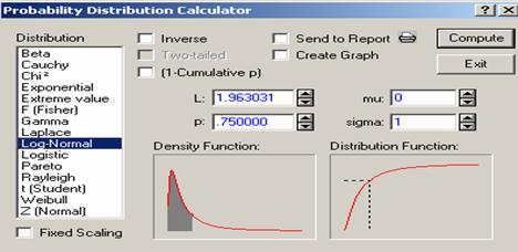
Figure 4.14 Probability Calculator for the Log-Normal Distribution
Similarly,
for the lognormal distribution with scale parameter m = 2 and shape parameter s = 5, one can
calculate ![]() by putting 2
for mu, 5 for sigma, 1.963031
for L, and click “compute” to get
0.395465 for p, i.e.,
by putting 2
for mu, 5 for sigma, 1.963031
for L, and click “compute” to get
0.395465 for p, i.e., ![]() .
.
The
Beta Probability Calculator
To
find the beta probability using Statistica, we select Beta from the
distribution list (See Figure 4.15).
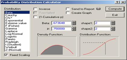
Figure 4.15 Probability Calculator for the Beta Distribution
By default, Statistica provides a Beta distribution
with parameters ![]() and
and ![]() . To calculate
. To calculate ![]() where X has a Beta distribution with parameters
2 and 2, put 0.673648 for Beta, click “compute” to get 0.75 for
where X has a Beta distribution with parameters
2 and 2, put 0.673648 for Beta, click “compute” to get 0.75 for ![]() , i.e.,
, i.e., ![]() .
.
Similarly
for a Beta distribution with shape parameter ![]() , and scale parameter
, and scale parameter ![]() , we can calculate
, we can calculate ![]() by putting 2 for the shape 1, 3 for the shape 2 and
0.673648 for Beta and click “compute” to get 0.894997 for p, i.e.,
by putting 2 for the shape 1, 3 for the shape 2 and
0.673648 for Beta and click “compute” to get 0.894997 for p, i.e., ![]() = 0.894997.
= 0.894997.
Exercises
4.1 The tread wear (in thousands of
kilometers) that car owners get with a certain kind of tire is a random
variable whose probability density is given by
![]()
(a)
Find the probability that one of
these tires will last at most 18000 kilometers.
(b)
Find the probability that one of
these tires will last anywhere from 27000 to 36000 kilometers.
(c)
Comment on the probability in (a)
if the
mean time to failure is b = 10000, 20000, 30000, 40000, 50000, 60000.
4.2 A
transistor has an exponential time to failure distribution with mean time to
failure of b = 20,000
hours.
(a)
What is the probability that the
transistor fails by 30,000 hours?
(b)
The transistor has already lasted
20, 000 hours in a particular application. What is the probability that it
fails by 30, 000 hours?
(c)
Comment on the probability in (a)
if ![]() .
.
4.3 The
lifetime X (in hours) of the central processing unit of a certain type of microcomputer is an exponential random
variable with parameter 0.001. What is the probability that the unit will work
at least 1,500 hours?
4.4 The lifetime (in hours) of the central processing unit of a
certain type of microcomputer is an exponential random variable with mean
β = 1000.
(a)
What is the probability that a
central processing unit will have a lifetime of at least 2000 hours?
(b) What is the
probability that a central processing unit will have a lifetime of at most 2000
hours
4.5 The
amount of raw sugar that one plant in a sugar refinery can process in one day
can be modeled as having an exponential
distribution with a mean of 4 tons. What is the probability that any
plant processes more than ![]() tons of sugar on a day?
tons of sugar on a day?
4.6 (Johnson,
R. A., 2000, 172). The amount of time that a surveillance camera will run
without having to be rested is a random variable having the exponential
distribution with ![]() days. Find the
probabilities that such a camera will
days. Find the
probabilities that such a camera will
(a) have to rested in less than 20 days;
(b) not have to rested in at least 60 days
4.7 (Johnson, R. A., 2000,
197). Consider a random variable having the exponential distribution with
parameter λ = 0.25. Find the probabilities that
(a) it takes values more than 200;
(b) it takes values less than 300.
4.8 (Johnson,
R. A., 2000, 168). If on the average three trucks arrive per hour to be
unloaded at a warehouse. Find the probability that the time between the
arrivals of successive trucks will be less than 5 minutes.
4.9 (Johnson,
R. A., 2000, 172). The number of weekly breakdowns of a computer is a random
variable having a Poisson distribution with λ = 0.3. Find the percent of
the time that the interval between the breakdowns of the computer will be
(a) less than one week;
(b) at least 5 weeks.
4.10 (Johnson, R. A., 2000,
173). Given that the switchboard of a consultant’s office receives on the
average 0.6 calls per minute. Find the probabilities that the time between the
successive calls arriving at the switchboard of the consulting firm will be
(a) less than ½ minute;
(b) more than 3 minutes.
4.11 Let
![]() have a standard normal distribution. Then evaluate the
following:
have a standard normal distribution. Then evaluate the
following:
![]()
![]()
![]()
![]()
![]()
![]()
![]() .
.
4.12 Solve
the following Probability equations to find normal percentiles:
![]()
![]()
![]()
![]()
![]()
![]()
![]()
![]()
![]() .
.
4.13 Complete the table where the ![]() ’s are the tail probabilities of the standard normal random
variable.
’s are the tail probabilities of the standard normal random
variable.
|
|
|
|
|
|
|
0.005 |
|
2.575829 |
|
|
|
|
|
|
|
|
|
|
|
2.170090 |
|
|
|
0.020 |
|
|
|
|
|
|
|
|
|
2.241403 |
|
0.050 |
|
|
|
|
|
|
|
|
|
1.644854 |
|
0.200 |
|
|
|
|
|
0.250 |
|
|
|
|
|
|
0.7 |
|
|
|
|
0.600 |
|
|
|
|
|
0.750 |
|
|
|
|
|
0.900 |
|
|
|
|
|
0.990 |
|
|
|
|
4.14 (cf. Devore, J. L., 2000, 171). Let ![]() denote the number of
flaws along a 100-m reel of magnetic tape. Suppose
denote the number of
flaws along a 100-m reel of magnetic tape. Suppose ![]() has approximately a
normal distribution with
has approximately a
normal distribution with ![]() and
and ![]() . Calculate the
probability that the number of flaws is
. Calculate the
probability that the number of flaws is
(a)
between
20 and 30.
(b)
at
most 30.
(c)
less
than 30.
(d)
not more than 25.
(e)
at
most 10
4.15 (Johnson,
R. A., 2000, 196). If a random variable has the standard normal distribution,
find the probability that it will take on a value
(a) between 0 and 2.50;
(b) between 1.22 and 2.35;
(c) between –1.33 and –0.33;
(d) between –1.60 and 1.80.
4.16 The length of each component in an assembly
is normally distributed with mean 6 inches and standard deviation ![]() inch. Specifications
require that each component be between 5.7 and 6.3 inches long. What proportion
of components will pass these requirements? Comment by varying
inch. Specifications
require that each component be between 5.7 and 6.3 inches long. What proportion
of components will pass these requirements? Comment by varying ![]() as
as
0.05 0.10
0.15 0.20 0.25
0.30 0.35 etc.
4.17 A machining operation produces steel shafts having diameters that
are normally distributed with a mean of 1.005 inches and a standard deviation
of 0.01 inch. Specifications call for diameters to fall within the interval
1.00 ![]() 0.02 inches.
0.02 inches.
(a)
What percentage of the output of this
operation will fail to meet specifications?
(b)
Comment on the percentage in (a)
if ![]() increases.
increases.
4.18 The weekly amount spent for maintenance and
repairs in a certain company has approximately a normal distribution with a
mean of $400 and a standard deviation of $20.
(a)
If $450 is budgeted to cover
repairs for next week, what is the probability that the actual costs will
exceed the budgeted amount?
(b) Comment on the
probability in part (a) if ![]() changes, keeping
changes, keeping ![]() fixed.
fixed.
(c) Comment on the
probability in part (a) if ![]() changes, keeping
changes, keeping ![]() fixed.
fixed.
4.19 A type of capacitor has resistance that
varies according to a normal distribution with a mean of 800 megohms and a standard
deviation of 200 megohms (Nelson, Industrial Quality Control, 1967, pp.
261-268). A certain application specifies capacitors with resistances between
900 and 1000 megohms. If 30 capacitors are randomly chosen from a lot of
capacitors of this type, what is the probability that at least 4 of them all
will satisfy the specification?
4.20 The fracture strengths of a certain type of
glass average 14 (in thousands of pounds per square inche) and have a standard
deviation of 1.9psi. What proportion of these glasses will have fracture
strength exceeding 14.5psi?
4.21 Suppose examination scores are normally
distributed with mean 60 and variance 25.
(a)
What value exceeds 25% of the
scores?
(b)
What value is exceeded by 25% of
the scores?
(c)
What is the minimum score to get
A+ if the top 3% students get A+?
(d)
What is the maximum score leading
to failure if the bottom 20% of students fails?
4.22 The life of a semi-conductor laser at a
constant power is normally distributed with a mean of 7000 hours and a standard
deviation of 600 hours.
(a)
What is the probability that the
laser fails before 5000 hours?
(b)
What is the life in hours that 5%
of the lasers exceed?
(c)
What life (in hours) is exceeded
by 5% of the lasers?
4.23 The
reaction time of a driver to visual stimulus is normally distributed with a
mean of 0.40 seconds and a standard deviation of 0.05 second.
(a)
What
is the probability that a reaction requires more than 0.50 second?
(b)
What
is the probability that a reaction requires between 0.4 and 0.5 second?
(c)
What
is the reaction time that is exceeded 90% of the time?
(d)
What
reaction time is exceeded 10% of the time?
4.24 The
personnel manager of a large company requires job applicants to take a certain
test and achieve a score of 500 or more. The test scores are distributed with mean 485 and
standard deviation 30. What score is exceeded
by 75% of the applicants? Assume that the test scores are normally distributed.
4.25 The
personnel manager of a large company requires employees to take a certain test.
The test scores are normally
distributed with mean 485 and standard deviation 30. The manager will
promote those applicants whose scores exceed 75th percentile, and
terminate those with scores less than 25th percentile.
(a) What is the minimum score to have promotion in the job?
(b) What is the maximum score for getting terminated from the job?
4.26 A Company produces light bulbs whose
lifetimes follow a normal distribution with mean 500 hours and standard
deviation 50 hours.
(a) If a light
bulb is chosen randomly from the company’s output, what is the probability that
its lifetime will be between 417.75 and 582.25 hours?
(b) If thirty
light bulbs are chosen at random, what is the probability that more than half
of them will survive more than the average lifetime?
4.27 ( Devore,
J. L., 2000, 164). The breakdown voltage of a randomly chosen diode of a
particular time is known to be normally distributed. What is the probability
that a diode’s breakdown voltage is within 1 standard deviation of its mean
value?
4.28 (Devore, J. L., 2000, 164).
The time that it takes a driver to react to the brake lights on a decelerating
vehicle is critical in helping to avoid rear-end collisions. The article
“Fast-Rise Brake Lamp as a Collision-Prevention Device” (Ergonomics, 1993:
391-395) suggests that reaction time for an in-traffic response to brake signal
from standard brake lights can be modeled with a normal distribution having
mean value 1.25 sec and standard deviation of .46 sec. What is the probability
that
(a) the reaction time is between 1.00 sec
and 1.75 sec?
(b) the reaction time exceeds 2 sec?
(c)
the reaction time is no more than 1.45 sec?
4.29 (Devore, J.
L., 2000, 169). Suppose that the force acting on a column that helps to support
a building is normally distributed with mean 15.0 kips and standard deviation
1.25 kips. What is the probability that the force
(a) is at most 17 kips?
(b) is between 10 and 12 kips?
(c) differs from 15 kips by at most 2
standard deviations?
4.30 (Johnson, R.
A., 2000, 197). The burning time of an experimental rocket is a random variable
having the normal distribution with mean = 4.76 seconds and standard deviation.
= 0.04 second. What is the probability that this kind of rocket will burn
(a) less than 4.66 seconds?
(b) more than 4.80 seconds?
(c) anywhere from
4.31 (Johnson, R.
A., 2000, 172). If a random variable has the gamma distribution with a = 2 and b = 2, find the probability that the random variable
will take on a value less than 4.
4.32 (Johnson, R. A., 2000,
172). In a certain city, the daily consumption of electric power (in millions
of kilowatt-hors) can be treated as a random variable having a gamma
distribution with a = 3 and b = 2. If the power plant of the city has a daily capacity of 12 million
kilowatt-hours, what is the probability that this power supply will be adequate
on any given day.
4.33 (Johnson, R. A., 2000,
171). Suppose that the lifetime of a certain kind of an emergency backup
battery (in hours) is a random variable ![]() having the Weibull distribution
with a = 0.1 and b = 0.5. Find
having the Weibull distribution
with a = 0.1 and b = 0.5. Find
(a) the probability that such a battery will
last more than 300 hours
(b) the probability that such a battery will
last less than 380 hours
(c) the probability that such a battery will
not last 100 hours.
4.34 (Johnson, R.
A., 2000, 173). Suppose that the time to failure (in minutes) of certain
electronic components subjected to continuous vibration may be looked upon as a
random variable having the Weibull distribution with a = 1/5 and b = 1/3. What is the probability that such a component
will fail in less than 5 hours?
4.35 (Johnson, R.
A., 2000, 173). Suppose that the service life (in hours) of a semiconductor is
a random variable having the Weibull distribution with a = 0.025 and b = 0.500. What is the probability that such a
semiconductor will still be in operating condition after 4,000 hours?
4.36 (Johnson, R.
A., 2000, 197). A mechanical engineer models the bending strength of a support
beam in a transmission tower as a random variable having the Weibull
distribution with a = 0.02 and b = 3.0. What is the probability that the beam can support a load of
4.5?
4.37 (Johnson, R. A., 2000,
169). In a certain country the proportion of highway sections requiring repairs
in any given year is a random variable with a = 3 and b = 2.
(a) On the average what percentage of the
highway sections requires repair in any given year?
(b) Find the probability that at most half
of the highway sections will require repair in any given year?
4.38 (Johnson, R. A., 2000, 173). If the annual
proportion of erroneous income tax returns filed with the IRS can be looked
upon as a random variable having a beta distribution with a = 2 and b = 9, what is the probability that in any given year
there will be fewer than 105 erroneous returns?
4.39 (Johnson, R. A., 2000,
173). Suppose that the proportion of the defectives shipped by a vendor, which
varies somewhat from shipment to shipment, is a random variable having the beta
distribution with a = 1 and b = 4. Find the probability that a shipment from this vendor will
contain 25% or more defectives.