CHAPTER THREE
Discrete Random Variables
The following are well known discrete
probability distributions.
Table 1 Discrete Probability Distributions
|
Distribution |
Probability function |
Mean |
Variance |
|
Binomial |
|
|
|
|
Geometric |
|
|
|
|
Hypergeometric |
|
|
|
Poisson
|
|
l |
l |


3.1 The Binomial Distribution
Example 3.1 An oil drilling company
ventures into various locations, and their success or failure is independent
from one location to another. Suppose the probability of a success at any
specific location is 0.1. If a driller drills 5 locations, find the probability
that there will be at least two successes.
Solution Let X be
the number of successful drilling of oils in 5 locations so that ![]() and
and

Computing Binomial
Probabilities Using Statistica
In Statistica, we compute binomial
probability using a function called Binom. This function
has three arguments; ![]() . The quantity x is the value assumed by the binomial
random variable X, whereas n and
p are respectively the number of
trials and probability of success. Thus,
to compute the binomial probability for Example 3.1, enter the numbers
0, 1, 2, 3, 4, 5 in one column, say VAR1.
Next, double-click another variable,
say VAR2 to obtain Figure 3.1.
. The quantity x is the value assumed by the binomial
random variable X, whereas n and
p are respectively the number of
trials and probability of success. Thus,
to compute the binomial probability for Example 3.1, enter the numbers
0, 1, 2, 3, 4, 5 in one column, say VAR1.
Next, double-click another variable,
say VAR2 to obtain Figure 3.1.
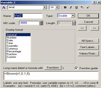
Figure 3.1 Result of Double Clicking a Variable
In the formula box at the bottom, write the
formula ![]() and click OK
and then Yes again for the Expression OK Dialogue
shown in Figure 3.2.
and click OK
and then Yes again for the Expression OK Dialogue
shown in Figure 3.2.
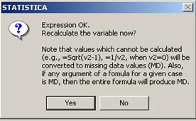
Figure
3.2 Expression OK
Dialogue
You will get the probability for each number
in Var1 and the Statistica will put the probability in Var2 as in Figure 3.3.
Then to solve the problem in Example 3.1, add the probabilities corresponding
to ![]() to
to ![]()
![]() .
.
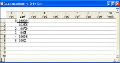
Figure 3.3 Probability Distribution of a Binomial Random Variable
To
solve Example 3.1 for cumulative
probabilities, one needs to go through the same steps as above and use the
function ![]() instead of
instead of ![]() .
.
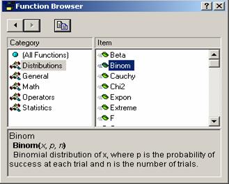
Instead
of typing in the functions, they can be selected from the Function
Browser. Double click the variable to get Figure 3.1. In the formula box
write “=” then click Functions to get the function browser shown
in Figure 3.4, then select Distributions under Category
on the left and Binom under Item on the right and
then press Enter to get the function ![]() in the formula box of
Figure 3.1. Next
in the formula box of
Figure 3.1. Next ![]() and n are replaced by their values and click
OK to get the final result in Var3.
and n are replaced by their values and click
OK to get the final result in Var3.
Figure
3.4 The Function Browser
Graphing the Binomial
Random Variable
To
plot a scatter graph for a binomial random variable, first create an appropriate
data sheet and enter the values of the sample space in one column. Next,
compute the binomial probabilities as above, then follow the steps:
1. Graphs/ 2D
Graphs/Scatter plots
2. In 2D Scatter plots
window, click Advanced
3. Choose Regular
for Graph Type and set Fit to off
4. Variables
(select the column containing the sample space as variable X and the column
containing the probability as variable ![]() ) / OK
) / OK
5. OK.
![]()
3.2
The Geometric Distribution
Example
3.2 A manufacturer uses electrical fuses in an
electronic system. The fuses are purchased in large lots and tested
sequentially until the first defective fuse is observed. Assume that the lot
contains 10% defective fuses. What is the probability that the
(a) first
defective fuse is observed on the first test?
(b) first
defective fuse is observed on the second test?
(c) first
defective fuse is observed on the third test?
Solution (a) ![]() (b)
(b) ![]() (c)
(c)![]() .
.
Computing Geometric
Probabilities Using Statistica
In Statistica, we compute
geometric probabilities using a function called Geom. This function has
two arguments: x and p.
The quantity x is the value assumed by the geometric random
variable X, and p is the
probability that a particular event (e.g., success) will occur. Thus, ![]()
is
used to compute the geometric probability for part (b) in Example 3.2. Double-click
any variable, say VAR2 to obtain the Figure 3.5.
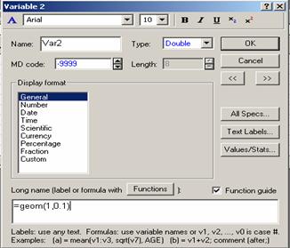
Figure 3.5 Result of
Double clicking a variable
Write
the formula ![]() in the formula box at
the bottom, and click OK and then Yes again for the Expression
OK Dialogue as shown in Figure 3.2 to get the answer (0.09) in all
cases in that variable (VAR2) as can be seen in Figure 3.6.
in the formula box at
the bottom, and click OK and then Yes again for the Expression
OK Dialogue as shown in Figure 3.2 to get the answer (0.09) in all
cases in that variable (VAR2) as can be seen in Figure 3.6.
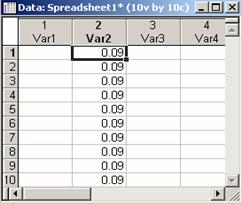
Figure
3.6 Result of “=Geom(1, 0.1)”
Note: We can also compute geometric probabilities using the Function Browser as in the case of binomial probabilities. Also cumulative probability can be calculated
using the function ![]() .
.
3.3
The Hypergeometric Distribution
Example
3.3 Suppose that a random sample of
size 2 is selected without replacement, from a lot of 100 laser printers and it is known that 5% of
the items in the lot are defective. What is the probability that
(a) none of them
is defective?
(b) one of them is
defective?
(c)
both are defective?
Solution:


3.4 The Poisson Distribution
Example 3.4 The number of failures of a
testing instrument from contamination particles on the product is a Poisson
random variable with a mean of 0.02 failures per hour.
(a) What is the
probability that the instrument does not fail in an 8-hour shift?
(b) What is the
probability of at least one failure in 30 minutes?
Solution
(a) Let ![]() = number of failures of the testing instrument per 8-hour
hour. Then the expected number of failures in an 8-hour shift is given by
= number of failures of the testing instrument per 8-hour
hour. Then the expected number of failures in an 8-hour shift is given by
![]()
so
that ![]() .
.
(b) Let ![]() = number of failures of the testing instrument in 30 minutes.
Then the expected number of failures in 30 minutes is given by
= number of failures of the testing instrument in 30 minutes.
Then the expected number of failures in 30 minutes is given by
![]()
so
that ![]() .
.
Computing Poisson
Probabilities Using Statistica
In Statistica, we compute Poisson probability using a function called Poisson. This function has two arguments: x and lambda (λ). The quantity x is the value assumed by the Poisson random variable X, and lambda (λ) is the expected value of x. Thus,
![]()
The
Poisson probability can be computed in the same way as for the binomial and geometric
distributions. To compute the Poisson probability ![]() for part (b) in Example 3.4, first compute
for part (b) in Example 3.4, first compute ![]() . Double click any variable, say VAR2, to obtain Figure 3.5
and in the formula box at the bottom, write the formula “= 1-Poisson (0, 0.01).” Click OK and
then Yes again for the Expression OK Dialogue as
shown in Figure 3.2, to get (0.009955) as in Figure 3.7. Cumulative
probabilities can also be calculated using the function
. Double click any variable, say VAR2, to obtain Figure 3.5
and in the formula box at the bottom, write the formula “= 1-Poisson (0, 0.01).” Click OK and
then Yes again for the Expression OK Dialogue as
shown in Figure 3.2, to get (0.009955) as in Figure 3.7. Cumulative
probabilities can also be calculated using the function ![]() .
.
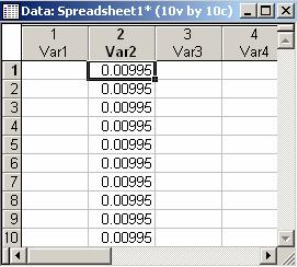
Figure 3.7 Result
of “=1-Poisson(0, 0.01)”
Note that we can also compute the Poisson
probabilities using the Function Browser
as done for the case of binomial.
Exercises
3.1
(Johnson,
R. A., 2000, 139). If the probability is 0.20 that a downtime of an automated
production process will exceed 2 minutes, find the probability that 3 of 8
downtimes of the process will exceed 2 minutes.
3.2
(Johnson,
R. A., 2000, 139). If the probability that a fluorescent light has a useful
life of at least 500 hours is 0.85, find the probabilities that among 20 such
lights
(a) 18 will have a useful life of at least 500 hours.
(b) at least 15 will have a useful life of at least
500 hours.
(c) at most 10 will not have a useful life of at least
500 hours.
3.3
(Johnson,
R. A., 2000, 125). It is known that 5% of the books bound at a certain bindery
have defective bindings. Find the probability that at least 20 of 100 books
bound by this bindery will have defective bindings.
3.4
(cf.
Devore, J. L., 2000, 123). Suppose that 20% of all copies of a particular
textbook fail a certain binding strength test. Let ![]() denote the number
among 15 randomly selected copies that fail the test. Then
denote the number
among 15 randomly selected copies that fail the test. Then ![]() has a binomial
distribution with
has a binomial
distribution with ![]() .
.
(a) Complete the probability and cumulative
probability distribution for the number of failures.
(b) Draw the probability and cumulative
probability histograms.
(c) Find the probability that at most 8 fail
the test.
(d) Find the probability that exactly 8 fail
the test.
(e) Find the probability that at least 8
fail.
(f) Find the probability that between 4 and
7, inclusive, fail the test.
3.5
(cf.
Devore, J. L., 2000, 123). An electronic manufacturer claims that 10% of its
power supply units need service during the warranty period. To investigate this
claim, technicians at a testing laboratory purchase 20 units and subject each
unit to accelerated testing to simulate use during the warranty period.
(a) Find the complete probability and
cumulative probability distributions for the number of units that need repair
during the warranty period.
(b) Draw the probability and cumulative
probability histograms.
(c) Find the probability that at most 6 need
repair during the warranty period.
(d) Find the probability that exactly 12
need repair during the warranty period.
(e) Find the probability that between 5 and
10, inclusive, need repair during the warranty period.
3.6
(cf.
Devore, J. L., 2000, 125). Compute the following binomial probabilities
(a) ![]() .
.
(b) ![]() when
when ![]() .
.
(c) ![]() when
when![]() .
.
(d) ![]() when
when ![]() .
.
(e) ![]() when
when ![]()
3.7
(cf.
Devore, J. L., 2000, 125). When circuit boards used in the manufacture of
compact disc players are tested, the long run percentage of defectives is 5%.
Let ![]() number of defective
boards in a random sample of size
number of defective
boards in a random sample of size ![]() . Determine:
. Determine:
(a) ![]() .
.
(b) ![]() .
.
(c) ![]() .
.
(d) What is the probability that none of the
35 boards are defective?
(e) Calculate the expected value and
standard deviation of ![]() .
.
3.8
(cf.
Devore, J. L., 2000, 125-126). A company that produces fine crystal knows from
experience that 10% of its goblets have cosmetic flaws and must be classified
as “seconds.”
(a) Among six randomly selected goblets, how
likely is it that only at least one is a second?
(b) Among six randomly selected goblets,
what is the probability that at least two are seconds?
(c) If goblets are examined one by one, what
is the probability that at most 5 of six are seconds?
3.9
(cf.
Devore, J. L., 2000, 126). Suppose that only 20% of all drivers come to a
complete stop at an intersection having flashing red lights in all directions
when no other cars are visible. What is the probability that, of 20 randomly
chosen drivers coming to an intersection under these conditions:
(a) at most 7 will come to a complete stop?
(b) more than 6 will come to a complete
stop?
(c) at least 8 will come to a complete stop?
(d) not all 20 will come to a stop?
3.10
(cf. Walpole, R. E, et. al, 2002, 134). In a
certain manufacturing process it is known that, on the average, 1 in every 100
items is defective. What is the probability that
(a) the fifth item inspected is the first
defective item found?
(b) at least four defective items are
checked before the first non defective item?
(c) at most four defective items are checked
before the first non defective item?
3.11
(cf.
Walpole, R. E, et. al, 2002, 135). At Busy time a telephone exchange is very
near capacity, so callers have difficulty placing their calls. It may be of
interest to know the number of attempts necessary in order to gain a
connection. Suppose that we let ![]() be the probability of
the connection during busy time. What is the probability that
be the probability of
the connection during busy time. What is the probability that
(a) 5 attempts are necessary for a successful call?
(b) 12 attempts are necessary for a successful call?
(c) 20 attempts are necessary for a successful call?
3.12
(cf. Walpole, R. E, et. al, 2002, 139). The
probability that a student pilot passes the written test for a private pilot’s
license is 0.7. Find the probability that the student will pass the test
(a) on the third try.
(b) on the seventh try.
(c) on the ninth try.
3.13
(Johnson,
R. A., 2000, 139). A basketball player makes 90% of his free throws. What
is the probability that he will miss for the first time on the seventh shot?
3.14
(cf.
Walpole, R. E, et. al, 2002, 137). During a laboratory experiment the average
number of radioactive particles passing through a counter in 1 millisecond is
4. What is the probability that
(a) 6 particles enter the counter in a given
millisecond?
(b) more than 8 particles enter the counter in a given
millisecond?
(c) no less than 2 particles enter the counter in a
given millisecond?
(d) less than 10 particles enter the counter in a
given millisecond?
3.15
(cf.
Walpole, R. E, et. al, 2002, 137). Ten is the average number of oil tankers
arriving each day at a certain port city. The facilities at the port can handle
at most 15 tankers per day. What is the probability that that on a given day
tankers have to be turned away?
3.16
(Walpole,
R. E, et. al, 2002, 139). On average, a certain intersection results in 3
traffic accidents per month. What is the probability that for any given month
at this intersection
(a) exactly 5 accidents will occur?
(b) less than 3 accidents will occur?
(c) at least 2 accidents will occur?
3.17
(Walpole,
R. E, et. al, 2002, 139). A secretary makes 2 errors per page on average. What
is the probability that on the next page, he will make
(a) 4 or more errors?
(b) no errors?
(c) less than 10 errors?
3.18
(Walpole,
R. E, et. al, 2002, 139). A certain area in the eastern
(a) fewer than 8 hurricanes.
(b) anywhere from 4 to 12 hurricanes.
(c) more than 10 hurricanes.
3.19
(Walpole,
R. E, et. al, 2002, 139). The average number of field mice per acre in a wheat
field is estimated to be 12. Find the probability that on a given acre
(a) fewer than 7 field mice are found.
(b) no less than 10 field mice are found.
(c) no fewer than 5 field mice are found.
3.20
(Johnson,
R. A., 2000, 128). If a bank receives on the average 6 bad checks per day, what
are the probabilities that it will receive
(a) 4 bad checks in any given day?
(b) 10 bad checks over any two consecutive days?
3.21
(Johnson,
R. A., 2000, 128). In the inspection of tinplate produced by a continuous
electrolytic process, 0.2 imperfections are spotted on the average per minute.
Find the probabilities of spotting
(a) one imperfection in 3 minutes.
(b) at least 2 imperfections in 5 minutes.
(c) at most one imperfection in 15 minutes.
3.22
(Johnson,
R. A., 2000, 131). Given that the switchboard of a consultant’s office receives
on the average 0.6 calls per minute. Find the probabilities that
(a) in a given minute, there will be at least 1 call.
(b) in a given minute, there will be at least 5 call.
3.23
(Johnson,
R. A., 2000, 131). At a checkout counter customers arrive at an average of 1.5
per minute. Find the probabilities that
(a) at most 4 will arrive in any given minute.
(b) at least 3 will arrive during an interval of 2
minutes.
(c) at most 15 will arrive during an interval of 6
minutes.
3.24
(Johnson,
R. A., 2000, 129). If on the average three trucks arrive per hour to be
unloaded at a warehouse, find the probability that at most 20 will arrive
during an 8-hour day shift.
3.25
(Johnson,
R. A., 2000, 140). The number of weekly breakdowns of a computer is a random
variable having a Poisson distribution with λ = 0.3. What is the
probability that the computer will operate without a breakdown for 2
consecutive weeks?
3.26 In a
shipment of 50 hard disks, five are defective. If four of the disks are
randomly selected for inspection, what is the probability that more than 2 are
defective?
3.27 A foundry ships engine blocks in lots of 20. Three items are
selected and tested. If the lot actually contains five defective items, find
the probability that there will be at least 2 defective blocks in the sample?
3.28 During the course of an hour 1000 bottles of soft drinks are
filled by a particular machine. Each hour a sample of 20 bottles is randomly
selected and the number of ounces of soft drink bottle is checked. Suppose that
during a particular hour 100 underfilled bottles are produced. What is the
probability that at least 3 underfilled bottles will be among those sampled?
3.29 Twenty microprocessor chips are in stock. Three have etching
errors that cannot be detected by the naked eye. Five chips are selected and
installed in field equipment. Find the probability that at least one chip with
an etching error will be chosen.
3.30 Production line workers assemble 15 automobiles per hour. During
a given hour, four are produced with improperly fitted doors. Three automobiles
are selected at random and inspected. Find the probability that at most one
will be found with improperly fitted doors.