The Big-O Notation – Introduction
Objectives
of this lecture
q Introduce the Big-O notation
q Learn how to analyze
Algorithms using the Big-O notation
q Apply the Big-O notation to
searching algorithms
Introduction
q Our main concern in
algorithm analysis is to find what happens to the running time of an algorithm
as the input data increases.
q One way of doing this is to
implement the various algorithms and run them on a computer with increasing
amount of data and record the time taken.
q However, this is clearly not
a very good method since the outcome would depend not only on the amount of
data but also on other factors such as the speed of the computer used and the
language of implementation
q A better method would be to express
the algorithm in terms of some mathematical representation (functions) and
analyze the resulting functions using mathematical tools.
q This is exactly what the
Big-O notation provides.
q The Big-O notation is a
functional analysis tool introduced by a German mathematician, Paul Bachmann in
1892- long before the development of computers
q The notation itself is very
simple and consist of the letter O, followed by a formula enclosed in
parenthesis as in O(n2) which is read as “Big-Oh of n squared”
q The Big-O of a function is obtained by simplifying the function to
obtain a much simpler function but which has the same behaviors as the original
function. This is done as follows:
Ø Eliminate any term whose
contribution to the total ceases to be significant as n becomes large-expressions
involving terms usually has one that dominates as n increases.
Ø Eliminate any constant
factors-constant factors have no effect on the overall patterns.
Definition
If f(n) and g(n) are functions defined on positive integers, then we write :
f(n) is O(g(n))
[read f(n) is Big-O of g(n)]
if
there exists a constant c such that
|f(n)| £ c|g(n)| for all sufficiently large positive integers n
Under these conditions, we say that “f(n)
has order at most g(n) or ‘f(n) grows no more rapidly than g(n)’
Examples
1. If f(n) = 100n, and wetake c=100, then we have
f(n) £ c(n) for
all n ³ 0
Thus, f(n) is O(n)
2. If f(n) =4n+200, and we take c=5, then we
obtain
f(n) £ c(n) for
all n ³ 200
Again, f(n) is O(n)
3. If f(n)=n2. Suppose we try to show
that f(n) is O(n). Doing so means that
we could find a constant c such that
n2 £ cn for
sufficiently large n
If we devide both sides by n, we have
n £ c for
sufficiently large n.
Clearly this is not true since c is a
constant.
Thus, n2 is not O(n)
- Sequential
Search
When analyzing algorithms, we normally take the worst case, which form the previous lecture we found to be n for sequential search.
i.e the performance of sequential search can be represented in terms of n as: f(n) = n
it obviously follows that f(n) is O(n)
Even if we take the average case:
f(n) =1/2(n+1)
We have f(n) £ n for
all n ³ 0
Thus f(n) is O(n).
- Binary
Search
The worst case we found from previous
lecture was log n
Thus the run time of binary search is
O(log n)
General
Observations
q The above examples of
polynomials generalize to the important rule about Big-O notation:
If f(n) is a polynomial in n with
degree r, then f(n) is O(nr), but f(n) is not O(ns) for any
s less than r.
q Another class of functions
that appear frequently in algorithm analysis are logarithms function. For these types of function, the following
rule applies:
Any logarithm of n grows more slowly (as n increases) than any positive power of n.
Thus, log n is O(nk)
And
nk is never O (log n) for k>O
Common
Orders
q When we apply the big-O
notation to algorithms, f(n) will normally be the running time and g(n) can be simplified using one
of the following notation.
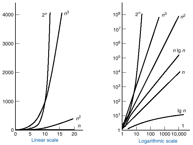
O(1) : computing time is constant (not dependent on n)
O(n) : computing time varies with n (linear)
O(n2) : quadratic
O(n3) : cubic
O(2n) : exponential
O(log n) : logarithmic
The table below shows the relative sizes of these numbers.
|
n |
log n |
n log n |
n2 |
n3 |
2n |
|
1 |
0.00 |
0 |
1 |
1 |
2 |
|
10 |
3.32 |
33 |
100 |
1000 |
1024 |
|
100 |
6.64 |
66 |
10,000 |
1,000,000 |
1.268x1030 |
|
1000 |
9.97 |
997 |
1,000,000 |
109 |
1.072x10301 |
q Notice how slower log n grows than n; This is essentially the
reason why binary search is superior to sequential search for large lists.
The following figure shows the growth rate of these functions
