CE317 Computer Methods
in CE
Lecture 1*: Mathematical and
Numerical Modeling
Introduction to the course:
Why do we need numerical methods?
Why is computer essential for numerical methods?
General steps
followed in numerical analysis
In
order to obtain a numerical solution for a problem in civil engineering or any
other field of science and engineering, one should follow the following general
six steps:
1-
Problem
definition:
State the problem verbally including the
process behavior, geometry, dimensions, known & unknown variables, and
simplifying assumptions.
2-
Mathematical
formulation:
Represent the information in step 1 by
functional relationship(s) usually algebraic or differential equation(s) using
fundamental laws and principals such as equilibrium.
3-
Numerical
formulation:
Approximate the above mathematical
formulation and develop a numerical procedure such that the problem can be
solved by simple repeated arithmetic operations.
4-
Computer
implementation:
The above numerical procedure is implemented
in a computer code to carry out the repeated calculations. Note that for
certain problems a computer package can be used where step 3 becomes
unnecessary.
5-
Verification
of the accuracy of the results:
The numerical results are checked against the
results of other analytical or numerical methods, if available. The convergence
of the solution can be checked using space or/and time mesh refinement.
6-
Interpretation
of computer output:
The obtained numerical output is used to
arrive at a decision. Sometimes this could be the hardest part of solving the
problem because it requires full understanding of the physical problems.
The
following simple example illustrates the use of the above four steps.
![]()
![]()
![]()
![]() Example 1: Flow of water in open channels
Example 1: Flow of water in open channels
![]() Flow rate = q
Flow rate = q
Velocity
of flow = v
Slope
of channel= s
h
Roughness
coefficient= n
![]() b
b
Given
q = 5 m3/s, b = 20 m, n= 0.03, s = 0.0002, determine the height of
water in the channel.
1-Problem definition:
It is required to determine the value of h corresponding to the following parameters: q = 5 m3/s, b = 20 m, n= 0.03, s = 0.0002
2-Mathematical Formulation:
We need to derive a mathematical relation between h and all other variables. From hydraulics, we know that the continuity equation is given by:
![]() (1)
(1)
The velocity is related to the cross-section geometry and slope through Manning equation:
![]() where
where
![]() (2)
(2)
Using (2) in (1), we get the
required relation:
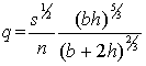 or
or 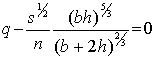
Using the given data, the above
equation becomes:
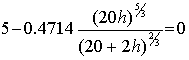 (3)
(3)
3-Numerical
Formulation & 4-Computer Implementation:
The root of eq. (3) is the
required value of h. We will learn in the first part of this course how to
obtain roots of all kinds of equations. The result for this equation is h =
0.7023 m.
5-
Verification of the accuracy of the results:
Using h = 0.7023 in (3), we get 0 = 0 O.K.
Example2: Deflection of a beam
![]()
 Determine the value and location of the
maximum deflection for the beam loaded as shown.
Determine the value and location of the
maximum deflection for the beam loaded as shown.
![]()
![]() W0
W0
![]()

L
Assume
that the beam is made of ASTM-A36 steel and has a w360x262 section.
1-Problem definition:
The load will deflect due to its own weight and the given triangular load. The shape of central line of the beam after deflection is called the elastic curve y(x). It is required to determine the value of x at which y(x) becomes maximum.
The following data is given:
the
intensity of the triangular load, w0 = 2 kN/m
the
length of the beam, L=4.5 m
From
Tables:
the
elastic modulus, E=200 N/mm2 for ASTM-A36 steel
the
moment of the inertia about the axis of bending (z-axix), Iz =849x106mm4
for w360x262.
Furthermore
let us assume that the self-weight of the beam is very small as compared to w0.
2-Mathematical Formulation:
From
CE203 we have learnt how to derive the equation of the elastic curve (which is
mainly based on equilibrium):
![]() where w0, E, Iz and L
are as given above.
where w0, E, Iz and L
are as given above.
In order to determine the location of maximum function y(x), we can set dy/dx=0 and determine the roots of the resulted polynomial, i.e.
![]()
One of the roots of the above equation corresponds to the required value of x.
3-Numerical
Formulation & 4-Computer Implementation:
There are several numerical
methods for computing the roots of polynomials that we are going to study in
this course. After doing the numerical analysis and computer implementation, we
obtain the following roots:
x1 =
-4.50 m, x2 = 4.50 m, x3 = -2.01 m and x4 =
2.01 m.
5-Interpretation
of the Computer Output:
The
two negative values are disregarded because x has to be a positive value
between 0 and 4.5 Furthermore the value of 4.5 is disregarded because the
deflection of the beam is zero at x=4.5 m (The beam is fixed at the right end).
We are left with x=2.01 m which is the location of the maximum deflection (ymax).
Therefore, ymax = y(2.01) = -0.049 m.